Bubble Sheet Multiple Choice Test with OpenCV and Python

In this tutorial, we are going to use OpenCV and Python to automatically read and grade bubble test sheets.

We will be using some techniques that we used in a previous tutorial when we created a simple document scanner.

The steps that we need to follow in order to build the project are:

1. Find the contours in the image.
2. Get the top-down view of the document using its contours.
3. Find the two biggest contours on the document.
4. Mask everything in the document except the area of the biggest contour.
5. Split the area of the biggest contour to get each answer in a box.
6. Go through each question and check if the user's answer is correct by comparing it to our list, which contains the indexes of the correct answers.

Find the Contours in the Image

First, create a new file named grader.py and put the following code:

import numpy as np
import cv2
from imutils.perspective import four_point_transform

from helper import show_images


# declare some variables
height = 800
width = 600
green = (0, 255, 0) # green color
red = (0, 0, 255) # red color
white = (255, 255, 255) # white color
questions = 5
answers = 5
correct_ans = [0, 2, 1, 3, 4]

We start by importing the required packages for the project and declare some useful variables.

You can see that we are importing the show_images function from the helper module which is not declared yet.

So let's create a new file named helper.py and put the code below inside it.

import cv2

def show_images(titles, images, wait=True):
    """Display multiple images with one line of code"""

    for (title, image) in zip(titles, images):
        cv2.imshow(title, image)

    if wait:
        cv2.waitKey(0)
        cv2.destroyAllWindows()

We will use this function later to display multiple images easily

The height and width variables will be used to resize our image using cv2.resize function.

The correct_ans variable is a bit important. This is a list containing the index of the correct answer for each question.

So, for example, correct_ans[1] will refer to the second question with the value 2 as the correct answer ("C").

In the image below, you can see all the correct answers marked in green:

Now, let's import our image and start processing it to find the contours:

img = cv2.imread('input/3.jpg')
img = cv2.resize(img, (width, height))
img_copy = img.copy() # for display purposes
img_copy1 = img.copy() # for display purposes

gray_img = cv2.cvtColor(img, cv2.COLOR_BGR2GRAY)
blur_img = cv2.GaussianBlur(gray_img, (5, 5), 0)
edge_img = cv2.Canny(blur_img, 10, 70)

# find the contours in the image
contours, _ = cv2.findContours(edge_img, cv2.RETR_LIST, cv2.CHAIN_APPROX_NONE)

# draw the contours
cv2.drawContours(img, contours, -1, green, 3)
show_images(['image'], [img]) # helper function in helper.py file

We import our image and resize it using the width and height we defined above.

Then we start preprocessing our image by converting it to grayscale, adding a little bit of blur, and detecting the edges by applying the Canny edge detector.

Finally, we apply the findContours function to find the contours in our edged image.

Below, you can see the contours applied to our image:

Obtain the Top-Down View of the Document

Now we want to get the top-down view of our document using the contours that we have found above.

I included this step in a function because we will use it again later.

def get_rect_cnts(contours):
    rect_cnts = []
    for cnt in contours:
        # approximate the contour
        peri = cv2.arcLength(cnt, True)
        approx = cv2.approxPolyDP(cnt, 0.02 * peri, True)
        # if the approximated contour is a rectangle ...
        if len(approx) == 4:
            # append it to our list
            rect_cnts.append(approx)
    # sort the contours from biggest to smallest
    rect_cnts = sorted(rect_cnts, key=cv2.contourArea, reverse=True)
    
    return rect_cnts

rect_cnts = get_rect_cnts(contours)
# warp perspective to get the top-down view of the document
document = four_point_transform(img_copy, rect_cnts[0].reshape(4, 2))
doc_copy = document.copy()  # for display purposes
doc_copy1 = document.copy() # for display purposes

cv2.drawContours(img_copy, rect_cnts, -1, green, 3)
# helper function in helper.py file
show_images(['image', 'document'], [img_copy, document])

We start looping over all the contours and approximate each contour. Then we check if the contour is a rectangle by checking if it has 4 points. If so, we put it in the rect_cnts list.

To make sure that our document's contour is the first in the list, we sort the contours from biggest to smallest (the document's contour is the biggest one in the image), and finally, we return the rect_cnts list.

Now that we have our list of contours, we apply the warp perspective to obtain the top-down view of our document. Note that we take the first contour from our list (rect_cnts[0]) which corresponds to the contour of the document.

In the image below, you can see the 'birds view' of the document:

Find the Two Biggest Contours on the Document

Now what we want to do is to take the top-down view of our document and find the contour of the questions and the contour of the grade. So we will apply the same steps as before:

# find contours on the document
gray_doc = cv2.cvtColor(document, cv2.COLOR_BGR2GRAY)
blur_doc = cv2.GaussianBlur(gray_doc, (5, 5), 0)
edge_doc = cv2.Canny(blur_doc, 10, 70)
contours, _ = cv2.findContours(edge_doc, cv2.RETR_EXTERNAL, cv2.CHAIN_APPROX_SIMPLE)

rect_cnts = get_rect_cnts(contours)
# outline of the questions
biggest_cnt = rect_cnts[0]
# outline of the grade
grade_cnt = rect_cnts[1]

# draw the two biggest contours, which are the 
# contour of the questions and the contour of the grade
cv2.drawContours(document, rect_cnts[:2], -1, green, 3)
show_images(['two biggest contours'], [document])

In order to find the contours in our document, we need to convert it to grayscale, blur it, and apply the Canny edge detector.

Then we use the function we defined above to get only the rectangle contours, sorted from biggest to smallest.

We finally take the contours of the questions and the grade from the list and put them in variables.

We are making the assumption that the contour of the questions is the biggest one, and the contour of the grade is the second biggest one in the document.

Below, you can see the two biggest contours in our document:

Mask Everything in the Document Except the Area of the Biggest Contour

Ok, now you need to pay attention because the interesting part starts here ...

In order to start grading our document, we want to hide everything in the image except the area of the questions.

Let's see how to do it:

# cooredinates of the biggest contour
# I added 4 pixels to x and y, and removed 4 pixels from x_W and y_H to make 
# sure we are inside the contour and not take the border of the biggest contour
x, y = biggest_cnt[0][0][0] + 4, biggest_cnt[0][0][1] + 4
x_W, y_H = biggest_cnt[2][0][0] - 4, biggest_cnt[2][0][1] - 4

# create a black image with the same dimensions as the document
mask =  np.zeros((document.shape[0], document.shape[1]), np.uint8)
# we create a white rectangle in the region of the biggest contour
cv2.rectangle(mask, (x, y), (x_W, y_H), white, -1) 
masked = cv2.bitwise_and(doc_copy, doc_copy, mask=mask)

show_images(['document', 'mask', 'masked'], [doc_copy, mask, masked])

We start by getting the coordinates of the contour of the questions because we need them when we apply our mask.

I added a few pixels to the coordinates to make sure that when we apply the mask we don't get the border of the contour, we only want the area inside the biggest contour.

Below, I included a screenshot to help you understand better:

After that, we create a black image of the same size as the document.

We use this black image to create a white rectangle on the region of interest (area of the questions)

We finally use the bitwise_and function to apply our mask to the document. By using our rectangle mask, we get only the area of the questions from the document.

Below you can see how we have focused only on the area of the biggest contour:

We are not done yet!

Now we want to get rid of the black part in the image and keep only the region of interest.

Since we have the coordinates of the biggest contour, we can just use NumPy slicing to achieve this:

# take only the region of the biggest contour
masked = masked[y:y_H, x:x_W]

and here is the result:

Finally, we convert the masked image to grayscale and apply thresholding to get a binary image:

gray = cv2.cvtColor(masked, cv2.COLOR_BGR2GRAY)
_, thresh = cv2.threshold(gray, 170, 255, cv2.THRESH_BINARY_INV)

show_images(['masked', 'thresh'], [masked, thresh])

Split the Area of the Biggest Contour

Now that we have focused only on the area of the questions, we want to split this region into 25 boxes, where each box contains a bubble answer.

Let's jump to the code to see how to do it:

# split the thresholded image into boxes
def split_image(image):
    # make the number of rows and columns 
    # a multiple of 5 (questions = answers = 5)
    r = len(image) // questions * questions 
    c = len(image[0]) // answers * answers
    image = image[:r, :c]
    # split the image horizontally (row-wise)
    rows = np.vsplit(image, questions)
    boxes = []
    for row in rows:
        # split each row vertically (column-wise)
        cols = np.hsplit(row, answers)
        for box in cols:
            boxes.append(box)
    return boxes

boxes = split_image(thresh)

We used a simple operation to make sure the dimensions of our thresholded image are always a multiple of 5 (number of questions and answers).

We need to do that because we are going to split our image into 5 equal parts (vertically and horizontally).

Then we use NumPy slicing to change the dimensions of the image.

So, for example, if we had an image with (257, 227) shape, after this operation it becomes (255, 225). We lose a few pixels, but that's ok.

Now we can split our image. We first split it horizontally using np.vsplit function to get the rows (the questions). Then we loop over the rows to split them vertically using np.hsplit function.

And finally, we put each box in our boxes list.

Below you can see a single box:

Start Grading the Document

In this last part, we are going to start the correction of the exam.

score = 0

# loop over the questions
for i in range(0, questions):
    user_answer = None
    
    # loop over the answers
    for j in range(answers):
        pixels = cv2.countNonZero(boxes[j + i * 5])
        # if the current answer has a larger number of 
        # non-zero (white) pixels then the previous one
        # we update the `user_answer` variable
        if user_answer is None or pixels > user_answer[1]:
            user_answer = (j, pixels)

 We initialize a score variable to keep track of the correct answer.

Then we start looping over the questions, and for each question, we loop over its answers.

After that, we need to check if the given answer is filled in or not. For that, we count the number of non-zero pixels of the current box using the cv2.countNonZero function. We can do this because the boxes in our boxes list are in the binary format (we used the thresh image to get the boxes).

Given the user's answer, we need to determine whether their answer is correct or not:

    # find the contours of the bubble that the user has filled
    cnt, _ = cv2.findContours(boxes[user_answer[0] + i * 5], 
                                      cv2.RETR_EXTERNAL, cv2.CHAIN_APPROX_SIMPLE)
    # translate the coordinates of the contours 
    # to their original place in the document
    for c in cnt:
        c[:, :, 0] += x + ((x_W - x) // 5) * user_answer[0]
        c[:, :, 1] += y + ((y_H - y) // 5) * i
        
    # if the user's answer is correct, we increase the score and draw
    # a green contour arround the bubble that the user has filled
    if correct_ans[i] == user_answer[0]:
        cv2.drawContours(doc_copy1, cnt, -1, green, 3)
        score += 1
    # otherwise we draw a red contour 
    else:
        cv2.drawContours(doc_copy1, cnt, -1, red, 3)

 We start by finding the contour of the user's answer using the boxes list.

We can't just draw the contours we found in our document, because we found the contours in the box image, not in the document. The coordinates are not the same for the two images.

So we need to translate the contours so that they will be in their original place in the document. That's what we are doing in the for loop.

Next, we check whether the user's answer is correct or not. In the case of a correct answer, we draw a green contour around its answer and increase the score variable by 1. However, if the answer is incorrect, we simply draw a red contour around it.

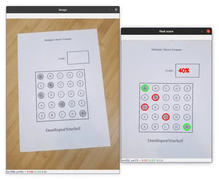
Finally, we format the score and display it inside the grade block:

score = (score / 5) * 100

# get the (x, y) coordinates of the grade contour.
# we add some pixels to make sure the text is inside the contour.
x_grade = grade_cnt[0][0][0] + 15
y_grade = grade_cnt[0][0][1] + 45
cv2.putText(doc_copy1, "{}%".format(int(score)), 
            (x_grade, y_grade), cv2.FONT_HERSHEY_SIMPLEX, 0.9, red, 3)

show_images(['image', 'final score'], [img_copy1, doc_copy1])

Below you can see a graded image with a  final score of 40%:

And here is another one with a  final score of 0%:

This one has a  final score of 100%:

Summary

In this tutorial, we learned how to build a bubble sheet scanner using optical mark recognition, Python, and OpenCV.

We used computer vision and image processing techniques to automatically read and grade a document.

If you want to learn more about computer vision and image processing then check out my course Computer Vision and Image Processing with OpenCV and Python.

You can get the source code for this article by clicking this link.

If you have any questions or want to say something, please leave a comment in the section below.