Convolutional Neural Network for Image Classification with Python and Keras

This picture is a derivative of "File:Typical cnn.png" by Aphex34 which is licensed under CC BY-SA 4.0

In deep learning, a convolutional neural network is a class of deep neural networks that have been used with great success in computer vision tasks such as image classification, object detection, image segmentation, ...

Neurons in a convolutional layer are not fully connected to every pixel in the input image like in a traditional neural network. Instead, they are connected to a small rectangle of pixels in the input image. 

In turn, each neuron in the second convolutional layer is connected only to other neurons located within a specific region in the first layer.

With this architecture, the model only has to focus on the tiny details in the first hidden layer such as edges, and then assemble these into more elaborated features in the second layer, and so on.

Moreover, this will make the convolutional neural network have much fewer parameters than a fully connected network which is useful to process large-size images.

The image below shows a typical CNN architecture:

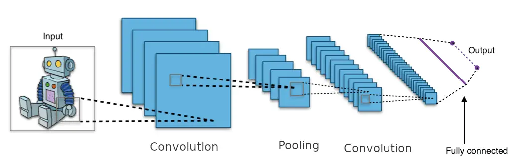
This picture is a derivative of "File:Typical cnn.png" by Aphex34 which is licensed under CC BY-SA 4.0

In this tutorial, we will see how to use a convolutional neural network to classify images from the Fashion MNIST and CIFAR-10 datasets.

In the previous tutorial, we built a fully connected neural network and we get around 88% on the validation set. You will see how a simple convolutional neural network will perform better than a fully connected layer.

Load Fashion MNIST

For convenience, we are going to load the dataset using the module tf.keras.datasets.

We will quickly redo the same steps as we did in the previous tutorial before building the convolutional neural network: import the datasets and scale the input features to the [0, 1] range before feeding them to the network.

from tensorflow import keras

fashion_mnist = keras.datasets.fashion_mnist
(X_full, y_full), (X_test, y_test) = fashion_mnist.load_data()

X_valid, X_train = X_full[:5000] / 255.0, X_full[5000:] / 255.0
y_valid, y_train = y_full[:5000], y_full[5000:]
X_test = X_test / 255.0

class_names = ["T-shirt/top", "Trouser", "Pullover", "Dress", "Coat", 
               "Sandal", "Shirt", "Sneaker", "Bag", "Ankle boot"]

We also need to reshape the data before feeding it to the network:

X_train = X_train.reshape((55000, 28, 28, 1))
X_valid = X_valid.reshape((5000, 28, 28, 1))
X_test = X_test.reshape((10000, 28, 28, 1))

Build a Simple Convolutional Neural Network

The common architecture of a convolutional neural network (CNN) generally takes a convolutional layer followed by a pooling layer then repeats the operation several times. A feedforward neural network is added on top of that, composed of a few densely connected layers and the last layer outputs the predictions.

The pooling layers are used to reduce the dimensions of the input image and thus reduce the number of parameters to learn, the computational load, and limit the risk of overfitting.

Below you can see what a basic convolutional neural network looks like:

from tensorflow.keras import Sequential
from tensorflow.keras.layers import Conv2D
from tensorflow.keras.layers import MaxPooling2D
from tensorflow.keras.layers import Dense
from tensorflow.keras.layers import Flatten


# build the model
model = Sequential([
    Conv2D(32, (3, 3), activation="relu", input_shape=(28, 28, 1), padding="same"),
    MaxPooling2D((2, 2)),
    Conv2D(64, (3, 3), activation="relu", padding="same"),
    MaxPooling2D((2, 2)),
    Conv2D(128, (3, 3), activation="relu", padding="same"),
    MaxPooling2D((2, 2)),
    Flatten(),
    Dense(64, activation="relu"),
    Dense(10, activation="softmax"),
])

model.summary()

# compile the model
model.compile(loss=keras.losses.SparseCategoricalCrossentropy(), 
              optimizer=keras.optimizers.SGD(), 
              metrics=[keras.metrics.SparseCategoricalAccuracy()])

# start training
epochs = 20
history = model.fit(X_train, y_train, epochs=epochs,
                    validation_data=(X_valid, y_valid))

A convolutional neural network (CNN) takes as input a tensor of shape (image_height, image_width, image_channels) without the batch dimension.

For the Fashion MNIST, the images are grayscale (image_channels = 1) images of 28 × 28 pixels.

The first Conv2D layer has 32 filter maps, each 3 x 3, using "same" padding and applying the ReLu activation function to its outputs. It is common to double the number of feature maps after each MaxPooling2D layer.

The MaxPooling2D layer uses a pool size of 2, which will divide the spatial dimensions by 2.

Here is the summary of the model:

Model: "sequential"
_________________________________________________________________
Layer (type)                 Output Shape              Param #   
=================================================================
conv2d (Conv2D)              (None, 28, 28, 32)        320       
_________________________________________________________________
max_pooling2d (MaxPooling2D) (None, 14, 14, 32)        0         
_________________________________________________________________
conv2d_1 (Conv2D)            (None, 14, 14, 64)        18496     
_________________________________________________________________
max_pooling2d_1 (MaxPooling2 (None, 7, 7, 64)          0         
_________________________________________________________________
conv2d_2 (Conv2D)            (None, 7, 7, 128)         73856     
_________________________________________________________________
max_pooling2d_2 (MaxPooling2 (None, 3, 3, 128)         0         
_________________________________________________________________
flatten (Flatten)            (None, 1152)              0         
_________________________________________________________________
dense (Dense)                (None, 64)                73792     
_________________________________________________________________
dense_1 (Dense)              (None, 10)                650       
=================================================================
Total params: 167,114
Trainable params: 167,114
Non-trainable params: 0
_________________________________________________________________

You can see from the model summary that the output of each Conv2D and MaxPooling2D layer is a 3D tensor (without the batch size) while a densely connected layer expects a 1D tensor.

That's why we need to flatten the 3D outputs to 1D (using the Flatten layer) before adding Dense layers on top. The Flatten layer takes the shape of the previous layer (None, 3, 3, 128) and multiplies the dimensions (3 x 3 x 128 = 1152).

The first Conv2D layer above has an output shape of (None, 28, 28, 32). The first dimension refers to the batch size.

The model doesn't know the batch size since we didn't specify it, so it is set to None.

When the training will start, if the batch size is unspecified, the fit method will set it to 32.

Now, let's take a look at the training of the model:

Epoch 1/20
1719/1719 [==============================] - 12s 3ms/step - loss: 1.4280 - sparse_categorical_accuracy: 0.4935 - val_loss: 0.6097 - val_sparse_categorical_accuracy: 0.7890
Epoch 2/20
1719/1719 [==============================] - 6s 3ms/step - loss: 0.5832 - sparse_categorical_accuracy: 0.7855 - val_loss: 0.4579 - val_sparse_categorical_accuracy: 0.8346
Epoch 3/20
1719/1719 [==============================] - 6s 3ms/step - loss: 0.4779 - sparse_categorical_accuracy: 0.8272 - val_loss: 0.4296 - val_sparse_categorical_accuracy: 0.8436
[...]
Epoch 18/20
1719/1719 [==============================] - 6s 3ms/step - loss: 0.2303 - sparse_categorical_accuracy: 0.9167 - val_loss: 0.2790 - val_sparse_categorical_accuracy: 0.8990
Epoch 19/20
1719/1719 [==============================] - 5s 3ms/step - loss: 0.2243 - sparse_categorical_accuracy: 0.9183 - val_loss: 0.2730 - val_sparse_categorical_accuracy: 0.9024
Epoch 20/20
1719/1719 [==============================] - 6s 3ms/step - loss: 0.2181 - sparse_categorical_accuracy: 0.9206 - val_loss: 0.2607 - val_sparse_categorical_accuracy: 0.9082

1719 represents the steps that the model needs to take before completing 1 epoch. Here's how it works: when training starts, we feed the training instances to the model. The model will process instances by what we call batches.

As I said above, when the batch size is not specified, it will be automatically set to 32. So the model will be fed the training instances by batches of 32 images each 28 x 28 pixels. 

Our training set contains 55,000 images. If we do the math, we have 55,000 images that will be fed to the network by batches of 32 images; how long will it take for the network to see all the images? 55,000 / 32 = 1718.75 steps ~ 1719 steps.

Let's take a look at the accuracy now. We get around 90.5% accuracy on the validation set after 20 epochs while we get 88.5% with a fully connected neural network (in the previous tutorial); that's a relative improvement of  17%. Not bad!

You can see that the model starts overfitting a bit (90.5% accuracy on the validation set vs 92% accuracy on the training set) but I want to stop here with the Fashion MNIST and introduce the CIFAR-10 dataset because this dataset is more challenging and overfitting will be our main issue.

You will see how the network will overfit the training data and what we can do to fight overfitting.

Load CIFAR-10

Again, for convenience, we are going to use tf.keras.datasets to load the dataset.

The dataset contains 60,000 color images of  32x32 pixels in 10 classes. There are 6000 images per class. The dataset is divided into a training set of 50,000 images and a test set of 10,000 images.

The classes in the dataset are: airplane, automobile, bird, cat, deer, dog, frog, horse, ship, truck.

Let's create a list that will contain the names of these classes:

class_names = ["airplane", "automobile", "bird", "cat", "deer", 
               "dog", "frog", "horse", "ship", "truck"]

and load the dataset:

cifar10 = keras.datasets.cifar10
(X_full, y_full), (X_test, y_test) = cifar10.load_data()

We need to create a validation set:

X_valid, X_train = X_full[:5000] / 255.0, X_full[5000:] / 255.0
y_valid, y_train = y_full[:5000], y_full[5000:]
X_test = X_test / 255.0

Let's plot some images from the training set with their labels:

import matplotlib.pyplot as plt

plt.figure(figsize=(8, 7))
for i in range(12):
    plt.subplot(3, 4, i+1)
    plt.xticks([])
    plt.yticks([])
    plt.imshow(X_train[i])
    plt.xlabel(class_names[y_train[i][0]])
plt.show()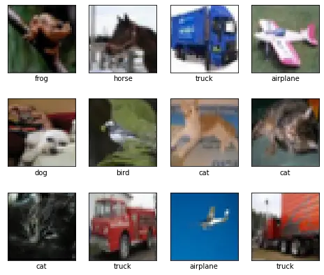

Build the CNN Model

We will follow the same general structure as above when we tackled the Fashion MNIST dataset: the convolutional neural network will be a stack of altered Conv2D and MaxPooling2d layers. Then a feedforward neural network will be added on top

But since the problem is more complex and challenging we will make the neural network deeper.

model = Sequential()
model.add(Conv2D(32, (3, 3), activation="relu", padding="same", input_shape=(32, 32, 3)))
model.add(MaxPooling2D((2, 2)))
model.add(Conv2D(64, (3, 3), activation="relu", padding="same"))
model.add(MaxPooling2D((2, 2)))
model.add(Conv2D(128, (3, 3), activation="relu", padding="same"))
model.add(MaxPooling2D((2, 2)))
model.add(Conv2D(256, (3, 3), activation="relu", padding="same"))
model.add(MaxPooling2D((2, 2)))
model.add(Flatten())
model.add(Dense(256, activation="relu"))
model.add(Dense(128, activation="relu"))
model.add(Dense(64, activation="relu"))
model.add(Dense(10, activation="softmax"))

Compile and Train the Model

We can now compile the model using the "sparse_categorical_crossentropy" loss function and the stochastic gradient descent ("sgd") algorithm for the optimizer.

model.compile(loss="sparse_categorical_crossentropy",
              optimizer="sgd",   
              metrics=["accuracy"])

We can start training just like we did with the Fashion MNIST. 

epochs = 25
history = model.fit(X_train, y_train, epochs=epochs,
                    validation_data=(X_valid, y_valid))

output: 

Epoch 1/25
1407/1407 [==============================] - 6s 4ms/step - loss: 2.2372 - accuracy: 0.1706 - val_loss: 1.9686 - val_accuracy: 0.3026
Epoch 2/25
1407/1407 [==============================] - 6s 4ms/step - loss: 1.7965 - accuracy: 0.3540 - val_loss: 1.6609 - val_accuracy: 0.3860
Epoch 3/25
1407/1407 [==============================] - 5s 4ms/step - loss: 1.5208 - accuracy: 0.4481 - val_loss: 1.4111 - val_accuracy: 0.4796
[...]
Epoch 22/25
1407/1407 [==============================] - 5s 4ms/step - loss: 0.1291 - accuracy: 0.9543 - val_loss: 1.3150 - val_accuracy: 0.7118
Epoch 23/25
1407/1407 [==============================] - 5s 4ms/step - loss: 0.1073 - accuracy: 0.9634 - val_loss: 1.8039 - val_accuracy: 0.6590
Epoch 24/25
1407/1407 [==============================] - 6s 4ms/step - loss: 0.1153 - accuracy: 0.9598 - val_loss: 1.5726 - val_accuracy: 0.6956
Epoch 25/25
1407/1407 [==============================] - 5s 4ms/step - loss: 0.0880 - accuracy: 0.9689 - val_loss: 1.5085 - val_accuracy: 0.7060

Visualizing Results

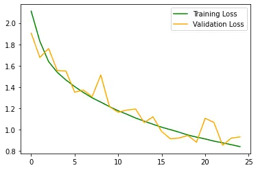
In the images below you can see the accuracy and the loss of the model on the training and validation set:

import matplotlib.pyplot as plt 


def plot_graph():
    acc = history.history['accuracy']
    val_acc = history.history['val_accuracy']

    loss = history.history['loss']
    val_loss = history.history['val_loss']

    plt.plot(range(epochs), acc, "b", label="Training Accuracy")
    plt.plot(range(epochs), val_acc, "r", label="Validation Accuracy")
    plt.legend()

    plt.figure()

    plt.plot(range(epochs), loss, "g", label="Training Loss")
    plt.plot(range(epochs), val_loss, "orange", label="Validation Loss")
    plt.legend()

    plt.show()

plot_graph()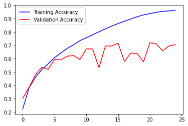

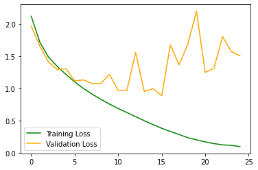
After 20 epochs, our validation accuracy hasn't exceeded 70%, meanwhile, our training accuracy continues to climb to more than 90%.

As you can see, the model didn't perform as well as with the Fashion MNIST. Also, notice how there is a big gap between the training accuracy and the validation accuracy: the model is clearly overfitting the training data.

There are several techniques that can help mitigate overfitting, such as dropout, regularization, obtain more data, data augmentation, etc.

In the next section, we will see what is data augmentation and how to apply it to the dataset.

Data Augmentation

Data augmentation is a technique used to artificially increase the size of a training dataset. It is the process of generating new training data that have similar characteristics to those already in the dataset.

This is done by augmenting the data via random transformations such as flipping, cropping to different sizes, rotating by different angles, etc.

This will allow the model to be more tolerant to small variations in images and generalize better.

There are several ways to apply data augmentation:

• We can use the ImageDataGenerator class
• We can use the Keras preprocessing layers
• We can write our own data augmentation pipelines using tf.data and tf.image (useful for finer control)

In this tutorial, we are going to use the Keras preprocessing layers.

There are two ways we can use these preprocessing layers: we can make them part of the model, or we can apply them directly to the dataset.

To learn more about the two options, please read the Two options to use the Keras preprocessing layers section of the Data augmentation tutorial.

In our case we are going to use the first option: make the preprocessing layers part of the model.

Let's see an example of data augmentation using the Keras preprocessing layers:

from tensorflow.keras.layers import RandomFlip
from tensorflow.keras.layers import RandomRotation
from tensorflow.keras.layers import RandomZoom
from tensorflow.keras.layers import RandomContrast

# for tensorflow version 2.5 or lower please use the code below instead
#from tensorflow.keras.layers.experimental.preprocessing import RandomFlip
#from tensorflow.keras.layers.experimental.preprocessing import RandomRotation
#from tensorflow.keras.layers.experimental.preprocessing import RandomZoom
#from tensorflow.keras.layers.experimental.preprocessing import RandomContrast


data_augmentation = Sequential([
    RandomFlip("horizontal", input_shape=(32, 32, 3)),
    RandomContrast(0.2),
    RandomRotation(0.1),
    RandomZoom(0.1),
])

In TensorFlow 2.5 or lower, some layers are still in the experimental module, like the one used for data augmentation. So if you are using TensorFlow version 2.5 or lower please use the commented code above.

You can check the version of TensorFlow using the commands below:

$ python3
>>> import tensorflow as tf
>>> tf.__version__
'2.6.0'

Here is the image to which we will apply data augmentation:

import matplotlib.pyplot as plt

plt.imshow(X_train[3])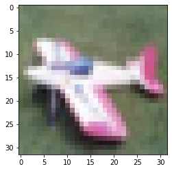

The image is a bit fuzzy, that's because the dataset contains images of 32 x 32 pixels each.

Let's see what the image will look like after applying data augmentation.

In the for loop below, after each iteration, a random transformation will be applied to the image before displaying the image.

import tensorflow as tf

# add the image to a batch.
# the shape of the image will be (1, 32, 32, 3)
image = tf.expand_dims(X_train[3], 0)

plt.figure(figsize=(10, 10))
for i in range(9):
    augmented_image = data_augmentation(image)
    plt.subplot(3, 3, i+1)
    plt.imshow(augmented_image[0])
    plt.axis("off")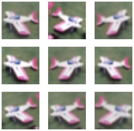

Let's create a new convolutional neural network using the augmented images:

model = keras.Sequential()
model.add(data_augmentation)
model.add(Conv2D(32, (3, 3), activation="relu", padding="same"))
model.add(MaxPooling2D((2, 2)))
model.add(Conv2D(64, (3, 3), activation="relu", padding="same"))
model.add(MaxPooling2D((2, 2)))
model.add(Conv2D(128, (3, 3), activation="relu", padding="same"))
model.add(MaxPooling2D((2, 2)))
model.add(Conv2D(256, (3, 3), activation="relu", padding="same"))
model.add(MaxPooling2D((2, 2)))
model.add(Flatten())
model.add(Dense(256, activation="relu"))
model.add(Dense(128, activation="relu"))
model.add(Dense(64, activation="relu"))
model.add(Dense(10, activation="softmax"))

model.compile(loss="sparse_categorical_crossentropy",
              optimizer="sgd",   
              metrics=["accuracy"])

epochs = 25
history = model.fit(X_train, y_train, epochs=epochs,
                    validation_data=(X_valid, y_valid))

output:

Epoch 1/25
1407/1407 [==============================] - 8s 5ms/step - loss: 2.2114 - accuracy: 0.1713 - val_loss: 1.9057 - val_accuracy: 0.3114
Epoch 2/25
1407/1407 [==============================] - 7s 5ms/step - loss: 1.8888 - accuracy: 0.3217 - val_loss: 1.6765 - val_accuracy: 0.3794
Epoch 3/25
1407/1407 [==============================] - 7s 5ms/step - loss: 1.6803 - accuracy: 0.3921 - val_loss: 1.7610 - val_accuracy: 0.4024
[...]
Epoch 22/25
1407/1407 [==============================] - 8s 6ms/step - loss: 0.8825 - accuracy: 0.6927 - val_loss: 1.0662 - val_accuracy: 0.6380
Epoch 23/25
1407/1407 [==============================] - 7s 5ms/step - loss: 0.8691 - accuracy: 0.6953 - val_loss: 0.8507 - val_accuracy: 0.7074
Epoch 24/25
1407/1407 [==============================] - 7s 5ms/step - loss: 0.8534 - accuracy: 0.7018 - val_loss: 0.9188 - val_accuracy: 0.6922
Epoch 25/25
1407/1407 [==============================] - 7s 5ms/step - loss: 0.8328 - accuracy: 0.7069 - val_loss: 0.9298 - val_accuracy: 0.6738

We get around 67% accuracy on the validation set and around 70.5% on the training set. We lost a bit of accuracy (we get 70.5% without data augmentation on the validation) but at least there is less overfitting than before.

You can see in the image below that training and validation accuracy are closer to each other:

plot_graph()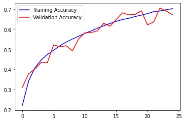

Evaluate the Model

Let's finish this tutorial by evaluating our trained model on the test set:

model.evaluate(X_test, y_test)
313/313 [==============================] - 1s 2ms/step - loss: 0.9619 - accuracy: 0.6677
[0.9618674516677856, 0.6676999926567078]

Resources and Further Reading

I will leave below some good resources if you want to learn more about convolutional neural networks and data augmentation. I personally used all of these resources to write this article:

Please note that some of these links are affiliate links, meaning I get a commission if you decide to make a purchase through my links, at no cost to you.

1. Part 2 Chapter 5 from the book Deep Learning with Python
2. Chapter 14 from the book Hands-On Machine Learning with Scikit-Learn, Keras, and TensorFlow
3. Convolutional Neural Network (CNN) tutorial from the TensorFlow platform
4. Data augmentation tutorial from the TensorFlow platform

If you want to learn machine learning and deep learning from scratch, I personally recommend the book Hands-On Machine Learning with Scikit-Learn, Keras, and TensorFlow. I personally read this book and found it extremely useful.

Summary

In today’s article, I showed you how to implement and train a simple convolutional neural network using Python and Keras. We used the Fashion MNIST and CIFAR-10 datasets.

Our simple convolutional neural network reached 90.82% accuracy on Fashion MNIST and 67.38% on CIFAR-10. It is not state of the art but we did much better than with a densely connected network.

In the next article, we will see how to use transfer learning and fine-tuning to further improve the accuracy of the model.

The final code used in this tutorial is available on GitHub in my repository.

You can also directly run the code on Google Colab.

If you have any questions or want to say something, please leave a comment in the section below.