Smile Detection with Python, OpenCV, and Deep Learning

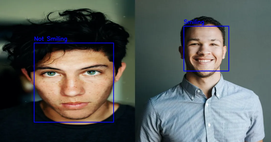
In this tutorial, we will use deep learning to build a more robust smile detector than the one we built in the previous tutorial where we used a Haar cascade smile detector.

We will use the SMILES dataset to train our convolutional neural network. Once our model is trained, we will follow the same steps as in the previous tutorial to detect smiles in images and videos:

• We will use Haar cascade to detect a face in an image.
• Extract the region of the face from the image.
• Pass the region of the face to our network for classification.
• Finally, we'll annotate the image with the text "Smiling" or "Not smiling" depending on the output of our network.

The SMILES dataset contains 13,165 grayscale images of  64x64 pixels in 2 classes: Smiling and Not smiling. There are exactly 9,475 images of "not smiling" faces and 3,690 images of "smiling" faces. The dataset is imbalanced, meaning that there is an uneven distribution of the images.

A common technique for dealing with an imbalanced dataset is to apply class weighting - we will see how to do it when we build our model.

You can download the dataset from here.

Loading the Data

Let's start by importing the required packages. Open a new file, name it training.py, and put the following code:

from sklearn.model_selection import train_test_split
from tensorflow.keras.preprocessing.image import img_to_array
from tensorflow.keras.utils import load_img
from tensorflow.keras import Sequential
from tensorflow.keras.layers import Conv2D
from tensorflow.keras.layers import MaxPool2D
from tensorflow.keras.layers import Flatten
from tensorflow.keras.layers import Dense
import numpy as np
import os 

Next, let's load our SMILES dataset:

valid_formats = [".jpg", ".jpeg", ".png"]

def image_paths(root):
    "get the full path to each image in the dataset"
    image_paths = []

    # loop over the diretory tree
    for dirpath, dirnames, filenames in os.walk(root):
        for filename in filenames:
            # extract the file extension from the filename
            extension = os.path.splitext(filename)[1].lower()

            # if the filename is an image we build the full 
            # path to the image and append it to our list
            if extension in valid_formats:
                image_path = os.path.join(dirpath, filename)
                image_paths.append(image_path)
    
    return image_paths

This function generates our image paths. It starts by exploring the directory tree and looks for each file. If the file is an image it will store the full path in a list.

Finally, it returns the image_paths list which contains the image paths.

We can now load our dataset:

image_paths = image_paths("SMILES")
IMG_SIZE = [32, 32]

def load_dataset(image_paths, target_size=IMG_SIZE):
    data = []
    labels = []
    
    # loop over the image paths
    for image_path in image_paths:
        # load the image in grayscale and convert it to an array
        image = load_img(image_path, color_mode="grayscale", target_size=target_size)
        image = img_to_array(image)
        # append the array to our list 
        data.append(image)
        
        # extract the label from the image path and append it to the `labels` list
        label = image_path.split(os.path.sep)[-3]
        label = 1 if label == "positives" else 0
        labels.append(label)
        
    return np.array(data) / 255.0, np.array(labels)

data, labels = load_dataset(image_paths, IMG_SIZE)

We get the list of our image paths using the image_paths() function passing it the root directory of our dataset.

Then inside the function load_dataset() we initialize two empty lists and loop over the image_paths list.

Here, we are using the load_img() function to load our image in grayscale and using a size of 32x32 pixels.

Next, we convert our image to an array and append it to the data list.

The label of each image is contained in the image path, so the next block of code extracts the label from the image path.

Positive samples (smiling faces) will be encoded 1 and negative samples (not smiling faces) will be encoded 0.

Here is an example of an image path and its corresponding label:

>>> image_path = "SMILES/negatives/negatives7/9975.jpg"
>>> image_path.split(os.path.sep)
['SMILES', 'negatives', 'negatives7', '9975.jpg']
>>> image_path.split(os.path.sep)[-3]
'negatives'

For this image path, the label will be encoded as 0. 

Finally, we append each label to the labels list, scale the pixel intensities to the [0, 1] range by dividing by 255.0, and return the data and labels arrays.

Next, let's build our model

Training the Smile Detector

The model we are going to build consists of a stack of two Conv2D + MaxPooling2D blocks, followed by a fully-connected layer with 256 units and using the ReLu activation function.

def build_model(input_shape=IMG_SIZE + [1]):
    model = Sequential([
        Conv2D(filters=32,
               kernel_size=(3, 3),
               activation="relu",
               padding='same',
               input_shape=input_shape),
        MaxPool2D(2, 2),
        Conv2D(filters=64,
               kernel_size=(3, 3),
               activation="relu",
               padding='same'),
        MaxPool2D(2, 2),
        Flatten(),
        Dense(256, activation="relu"),
        Dense(1, activation="sigmoid")
    ])

    model.compile(loss="binary_crossentropy", optimizer="adam", metrics=["accuracy"])
    return model

Since we are dealing with a binary classification problem (2 classes) we are using the sigmoid activation function and a single neuron in the output layer.

Next, we need to calculate the class weights. As I said before, our dataset is imbalanced so we need to give more weight to the under-represented class (the "smiling" class in this case) so that the model will pay more attention to this class.

# count the number of each label 
label, counts = np.unique(labels, return_counts=True)
# compute the class weights
counts = max(counts) / counts
class_weight = dict(zip(label, counts))

Here, label and counts are set to: [0, 1] and [9475, 3690] respectively.

Next, we compute the weight for each class and create a dictionary that maps each class with its weight. The class_weight variable will be set to: {0: 1.0, 1: 2.567750677506775}.

You can learn more about imbalanced data here: Classification on imbalanced data. 

Now we need to create a train set, a validation set, and a test set. we will take 20% of the data to create the test set and from the remaining 80% we will take 20% to create the validation set:

(X_train, X_test, y_train, y_test) = train_test_split(data, labels, 
                                                    test_size=0.2,
                                                    stratify=labels,
                                                    random_state=42)

(X_train, X_valid, y_train, y_valid) = train_test_split(X_train, y_train,
                                                        test_size=0.2,
                                                        stratify=y_train,
                                                        random_state=42)

 Finally, we can build our network and start training:

# build the model
model = build_model()

# train the model
EPOCHS = 20
history = model.fit(X_train, y_train,
                    validation_data=(X_valid, y_valid),
                    class_weight=class_weight,
                    batch_size=64,
                    epochs=EPOCHS)

# save the model
model.save("model")

We make sure to save our model to test it later in some images and videos.

output:

Epoch 1/20
132/132 [==============================] - 4s 7ms/step - loss: 0.7143 - accuracy: 0.7334 - val_loss: 0.3311 - val_accuracy: 0.8647
Epoch 2/20
132/132 [==============================] - 1s 4ms/step - loss: 0.4341 - accuracy: 0.8772 - val_loss: 0.3070 - val_accuracy: 0.8804
...
Epoch 19/20
132/132 [==============================] - 1s 4ms/step - loss: 0.1353 - accuracy: 0.9658 - val_loss: 0.3039 - val_accuracy: 0.9070
Epoch 20/20
132/132 [==============================] - 1s 5ms/step - loss: 0.1264 - accuracy: 0.9659 - val_loss: 0.3365 - val_accuracy: 0.9037

Let's also plot the learning curves of the training and validation accuracy/loss:

import matplotlib.pyplot as plt

acc = history.history['accuracy']
val_acc = history.history['val_accuracy']

loss = history.history['loss']
val_loss = history.history['val_loss']

plt.plot(range(EPOCHS), acc, "b", label="Training Accuracy")
plt.plot(range(EPOCHS), val_acc, "r", label="Validation Accuracy")
plt.legend()

plt.figure()

plt.plot(range(EPOCHS), loss, "g", label="Training Loss")
plt.plot(range(EPOCHS), val_loss, "orange", label="Validation Loss")
plt.legend()

plt.show()

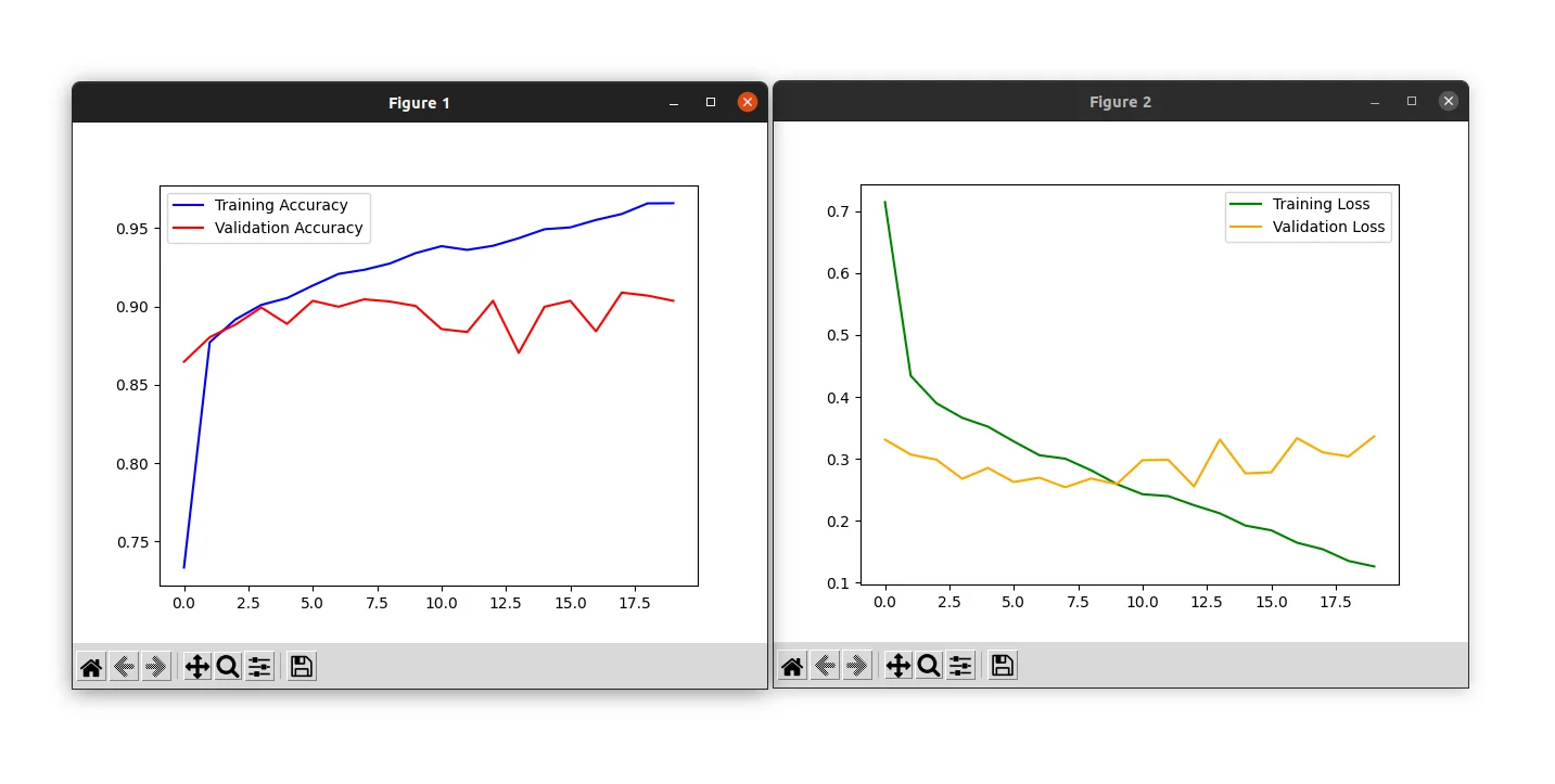
We achieved a validation accuracy of 90% but you can notice that the training and validation loss start to diverge past epoch 10: this is a sign of overfitting.

If you want to learn more about overfitting and how to avoid it, please refer to the Overfitting and Underfitting in Deep Learning tutorial.

Let's evaluate the model on the test set:

# Evaluate the model on the test set
test_loss, test_accuracy = model.evaluate(X_test, y_test)
print(f'Test Loss: {test_loss:.4f}, Test Accuracy: {test_accuracy * 100:.2f}%')

output:

83/83 [==============================] - 0s 2ms/step - loss: 0.2613 - accuracy: 0.9062
Test Loss: 0.2613, Test Accuracy: 90.62%

After 20 epochs, you can see that the network achieved 90% accuracy on the test set.

Applying Our Smile Detector to Images

Now that our model is trained, let's apply it to some real-world images. Create a new Python file named smile_detector_image.py and let's write some code:

import cv2
from keras.models import load_model
import numpy as np


width = 800
height = 600
blue = (255, 0, 0)

# load the image, resize it, and convert it to grayscale
image = cv2.imread("images/1.jpg")
image = cv2.resize(image, (width, height))
gray = cv2.cvtColor(image, cv2.COLOR_BGR2GRAY)

Here we are importing the required packages and then loading our image, resizing it, and converting it to grayscale.

Next, let's detect faces using a Haar cascade classifier:

# load the haar cascade face detector
face_detector = cv2.CascadeClassifier("haar_cascade/haarcascade_frontalface_default.xml")
# load our trained model
model = load_model("model")

# detect faces in the grayscale image
face_rects = face_detector.detectMultiScale(gray, 1.1, 8)

The haarcascade_frontalface_default.xml file is provided with the source code of this tutorial, make sure to download it.

The face_rects variable will contain the face bounding boxes.

So the next step is to loop over the face bounding boxes:

# loop over the face bounding boxes
for (x, y, w, h) in face_rects:
    cv2.rectangle(image, (x, y), (x + w, y + h), blue, 2)
    # extract the region of the face from the grayscale image
    roi = gray[y:y + h, x:x + w]
    roi = cv2.resize(roi, (32, 32))
    roi = roi / 255.0
    # add a new axis to the image
    # previous shape: (32, 32), new shape: (1, 32, 32)
    roi = roi[np.newaxis, ...]

We are using the coordinates of each bounding box to draw a rectangle around the face, and extract the region of the face from the image.

We also need to resize the face region to 32x32 pixels, scale it, and add a new dimension so that we can pass it to our network.

Finally, we can pass the region of the face through the network for classification:

    # apply the smile detector to the face roi
    prediction = model.predict(roi)[0]
    label = "Smiling" if prediction >= 0.5 else "Not Smiling"

The prediction will have a value between 0 and 1. If the prediction is equal to or greater than 0.5 we set the label to "Smiling", otherwise, we set it to "Not smiling".

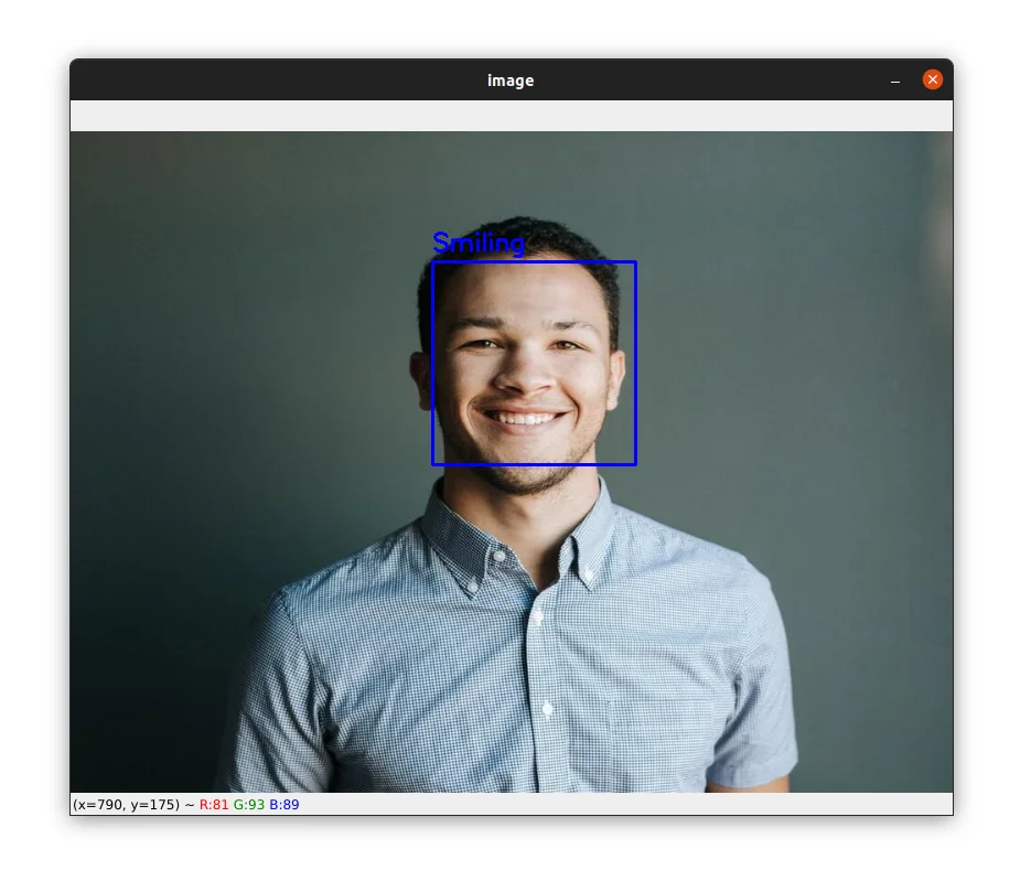
We can now write the label on the image and display the image:

    cv2.putText(image, label, (x, y - 10), cv2.FONT_HERSHEY_SIMPLEX,
            0.75, blue, 2)
cv2.imshow("image", image)
cv2.waitKey(0)

The image below shows a detection of smiling:

And here is an example of not smiling:

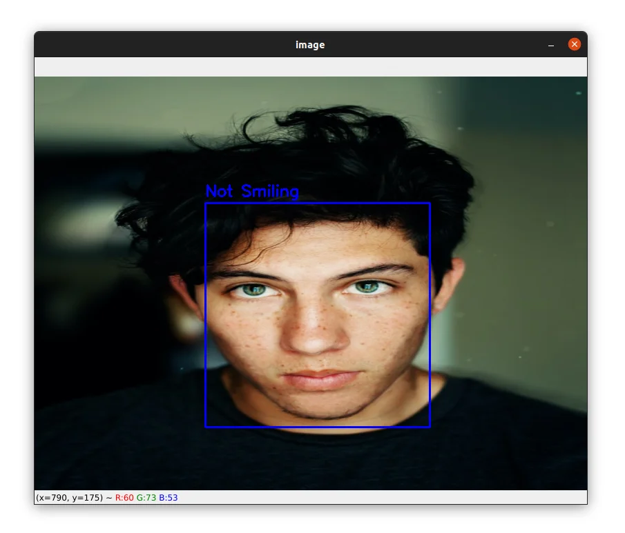
Other images are available with the source code, make sure to test with them too.

Let's now test our model in a video.

Applying Our Smile Detector to Videos

Now that you know how to detect smiles in images, let's see how to apply our deep learning smile detector to videos.

Open a new file, name it smile_detection_video.py, and write the following code:

import cv2
from keras.models import load_model
import numpy as np

blue = (255, 0, 0)

video_capture = cv2.VideoCapture(0)

# load the haar cascade face detector
face_detector = cv2.CascadeClassifier("haar_cascade/haarcascade_frontalface_default.xml")
# load our trained model
model = load_model("model")

We first import our required packages. We then initialize the video capture and load our face and smile detectors.

Let's now process our frames to apply our Haar cascade face detector:

# loop over the frames
while True:
    # get the next frame from the video and convert it to grayscale
    _, frame = video_capture.read()
    gray = cv2.cvtColor(frame, cv2.COLOR_BGR2GRAY)
    
    # apply our face detector to the grayscale frame
    faces = face_detector.detectMultiScale(gray, 1.1, 8)

We grab the next frame from the video capture and convert it to grayscale.

Next, we perform face detection using the Haar cascade face detector.

Now, we can loop over the face bounding boxes:

    # go through the face bounding boxes 
    for (x, y, w, h) in faces:
        # draw a rectangle around the face on the frame
        cv2.rectangle(frame, (x, y), (x + w, y + h), blue, 2)
        # extract the face from the grayscale frame
        roi = gray[y:y + h, x:x + w]
        roi = cv2.resize(roi, (32, 32))
        roi = roi / 255.0
        # add a new axis to the image
        # previous shape: (32, 32), new shape: (1, 32, 32)
        roi = roi[np.newaxis, ...]
        # apply the smile detector to the face roi
        prediction = model.predict(roi)[0]
        label = "Smiling" if prediction >= 0.5 else "Not Smiling"

This block of code is the same as in the previous section where we perform smile detection in images except that we are applying smile detection to a frame instead of an image.

Finally, we can now write the label on the frame and display the frame:

        cv2.putText(frame, label, (x, y - 10), cv2.FONT_HERSHEY_SIMPLEX,
                0.75, blue, 2)
         
                
    cv2.imshow('Frame', frame)
   
    # wait for 1 milliseconde and if the q key is pressed, we break the loop
    if cv2.waitKey(1) == ord('q'):
        break
    
# release the video capture and close all windows
video_capture.release()
cv2.destroyAllWindows()

As you can see in the video above, the brightness of the face influences the detection of the smile, especially since in the case of this video my face is underexposed.

The algorithm has trouble detecting "smiling" from "non-smiling" but when I point a light towards my face you can see that the detection is correct.

To workaround this problem we can implement adaptive histogram equalization to adjust the contrast of the face.

With OpenCV, this means adding just two lines of code to our program. We have the OpenCV's cv2.createCLAHE function to apply adaptive histogram equalization.

Here is how to do it:

    # go through the face bounding boxes 
    for (x, y, w, h) in faces:
        # draw a rectangle around the face on the frame
        cv2.rectangle(frame, (x, y), (x + w, y + h), blue, 2)
        # extract the face from the grayscale image
        roi = gray[y:y + h, x:x + w]

        # Applying CLAHE to the face ROI
        clahe = cv2.createCLAHE(clipLimit=2.5, tileGridSize=(8,8))
        roi_clahe = clahe.apply(roi)
        cv2.imshow("CLAHE", roi_clahe)
        
        # ...
            
    cv2.imshow('Frame', frame)
    # ...
# ...

The cliplimit argument is the threshold for contrast limiting and the tileGridSize argument specifies the size of the tiles that will be used to apply histogram equalization.

The apply method applies CLAHE (Contrast Limited Adaptive Histogram Equalization) and equalizes the histogram of the grayscale face ROI.

The result of this simple image processing technique can be shown in the video below:

As you can see, this time the algorithm has no problem detecting smiling and non-smiling from the video and the detection is quite stable.

Summary

In this tutorial, you learned how to train a convolutional neural network to detect smiling in images and videos.

The first thing we had to do is to load our dataset from disk and prepare it for our network.

Next, we created our neural network and calculated the class weights to account for class imbalance in the dataset and thus force the model to pay more attention to the under-represented class.

We then split our dataset into a training set, a validation set, and a test set and then proceed to train our model. We achieved an accuracy of 90% on the test set.

The final step was to test our model in images and videos. For that, we used a Haar cascade face detector to detect a face in the image, extract the face from the image, and pass the face ROI to our model to label it as "Smiling or "Not smiling".

If you want to learn more about computer vision and image processing then check out my course Computer Vision and Image Processing with OpenCV and Python.

You can get the source code for this article by clicking this link.

If you have any questions or want to say something, please leave a comment in the section below.

Related Tutorials

Here are some related tutorials that you may find interesting:

1. Face Detection and Blurring with OpenCV and Python

2. Eye Blink Counter with Dlib, Python, and OpenCV

3. Smile Detection with Python, OpenCV, and Haar Cascade

4. Face Recognition with Python, Dlib, and Deep Learning

5. How to Detect Face landmarks with Dlib, Python, and OpenCV