Overfitting and Underfitting in Deep Learning

There are two major problems when training neural networks: overfitting and underfitting.

Overfitting is a problem that can occur when the model is too sensitive to the training data. The model will then fail to generalize and perform well on new data. This can happen when there are too many parameters in the model.

This is noticeable in the learning curve by a big gap between the training and validation loss/accuracy.

Underfitting is the opposite of overfitting. It occurs when the model is not sensitive enough to the training data and as a result, the model fails to learn the most important patterns in the training data.

Underfitting is often not really a problem because you can prevent it by simply making your model more deep (add more layers/neurons to the model) or training for a few more epochs.

There are two main ways to avoid overfitting: gather more training data and apply regularization techniques to penalize the model.

Let's see an example by training a convolutional neural network on the CIFAR-10 dataset.

Load the Dataset

Let's first download the data:

from tensorflow.keras.datasets import cifar10


(X_train, y_train), (X_test, y_test) = cifar10.load_data()

Build and Train the model

The model we are going to build consists of a stack of two Conv2D + Conv2D + MaxPooling2D blocks, followed by a fully-connected layer with 256 units and using the ReLu activation function.

from tensorflow.keras.models import Sequential
from tensorflow.keras.layers import Conv2D
from tensorflow.keras.layers import Flatten
from tensorflow.keras.layers import Dense
from tensorflow.keras.layers import MaxPooling2D
from tensorflow.keras.layers import Rescaling


model = Sequential([
    Rescaling(1./255, input_shape=(32, 32, 3)),
    Conv2D(32, 3, padding="same", activation="relu"),
    Conv2D(32, 3, padding="same", activation="relu"),
    MaxPooling2D(pool_size=(2, 2)),
    Conv2D(64, 3, padding="same", activation="relu"),
    Conv2D(64, 3, padding="same", activation="relu"),
    MaxPooling2D(pool_size=(2, 2)),
    Flatten(),
    Dense(256, activation="relu"),
    Dense(10, activation="softmax")
])

Here you can see that we are using tf.keras.layers.Rescaling to scale the data to the range [0, 1]; each input image will be multiplied by 1./255.

Let's compile our model and start training:

model.compile(
    optimizer="Adam",
    loss="sparse_categorical_crossentropy",
    metrics=["accuracy"],
)

epochs = 30

history = model.fit(
    X_train, y_train,
    validation_data=(X_test, y_test),
    epochs=epochs,
    batch_size=64,
)

output:

Epoch 1/30
782/782 [==============================] - 11s 8ms/step - loss: 1.3713 - accuracy: 0.5065 - val_loss: 1.0902 - val_accuracy: 0.6244
Epoch 2/30
782/782 [==============================] - 4s 6ms/step - loss: 0.9214 - accuracy: 0.6755 - val_loss: 0.8700 - val_accuracy: 0.6945
...
Epoch 29/30
782/782 [==============================] - 5s 7ms/step - loss: 0.0524 - accuracy: 0.9833 - val_loss: 2.4223 - val_accuracy: 0.7356
Epoch 30/30
782/782 [==============================] - 6s 7ms/step - loss: 0.0398 - accuracy: 0.9866 - val_loss: 2.4421 - val_accuracy: 0.7253

Visualize the Results

Let's plot the loss and accuracy curves for the training and validation sets:

import matplotlib.pyplot as plt


def plot_learning_curves():
    accuracy = history.history["accuracy"]
    val_accuracy = history.history["val_accuracy"]

    loss = history.history['loss']
    val_loss = history.history['val_loss']

    plt.figure(figsize=(8, 8))
    plt.subplot(2, 1, 1)
    plt.plot(range(epochs), accuracy, label='Training Accuracy')
    plt.plot(range(epochs), val_accuracy, label='Validation Accuracy')
    plt.legend(loc='lower right')
    plt.title('Training and Validation Accuracy')

    plt.subplot(2, 1, 2)
    plt.plot(range(epochs), loss, label='Training Loss')
    plt.plot(range(epochs), val_loss, label='Validation Loss')
    plt.legend(loc='upper left')
    plt.title('Training and Validation Loss')
    plt.show()

plot_learning_curves()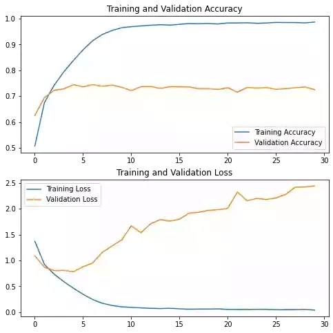

As you can in the plot above, there is a big gap between the training and validation loss/accuracy: we are clearly overfitting. It's normal though to have a small gap between them and our goal is to reduce and limit this gap as much as possible.

Reduce Overfitting with Dropout

Dropout is a popular regularization technique for neural networks.

When applied to a layer, every neuron in this layer has a probability p of being dropped out (by setting its activation to zero) during training. The dropout rate p is generally set between 0.2 and 0.5 meaning that 20% to 50% of neurons in the layer will be deactivated.

Let's add a Dropout layer after each MaxPooling2D layer:

from tensorflow.keras.layers import Dropout

model = Sequential([
    Rescaling(1./255, input_shape=(32, 32, 3)),
    Conv2D(32, 3, padding="same", activation="relu"),
    Conv2D(32, 3, padding="same", activation="relu"),
    MaxPooling2D(pool_size=(2, 2)),
    Dropout(0.5),
    Conv2D(64, 3, padding="same", activation="relu"),
    Conv2D(64, 3, padding="same", activation="relu"),
    MaxPooling2D(pool_size=(2, 2)),
    Dropout(0.5),
    Flatten(),
    Dense(256, activation="relu"),
    Dense(10, activation="softmax")
])

model.compile(
    optimizer="Adam",
    loss="sparse_categorical_crossentropy",
    metrics=["accuracy"],
)

epochs = 30

history = model.fit(
    X_train, y_train,
    validation_data=(X_test, y_test),
    epochs=epochs,
    batch_size=64,
)

output:

Epoch 1/30
782/782 [==============================] - 6s 7ms/step - loss: 1.5553 - accuracy: 0.4319 - val_loss: 1.1631 - val_accuracy: 0.5812
Epoch 2/30
782/782 [==============================] - 6s 7ms/step - loss: 1.1456 - accuracy: 0.5878 - val_loss: 1.0058 - val_accuracy: 0.6407
...
Epoch 29/30
782/782 [==============================] - 5s 6ms/step - loss: 0.3501 - accuracy: 0.8735 - val_loss: 0.7083 - val_accuracy: 0.7848
Epoch 30/30
782/782 [==============================] - 6s 8ms/step - loss: 0.3453 - accuracy: 0.8767 - val_loss: 0.7189 - val_accuracy: 0.7825

plot_learning_curves()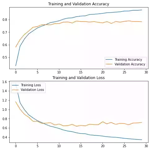

You can see that after applying dropout, there is less overfitting than before.

Let's now try data augmentation to see if that will help us combat overfitting even more.

Reduce Overfitting with Data Augmentation

Data augmentation is another regularization technique that artificially increases the size of a dataset by applying random transformations such as flipping, cropping to different sizes, rotating by different angles, etc.

In Keras, there are several preprocessing layers for that:

from tensorflow.keras.layers import RandomFlip
from tensorflow.keras.layers import RandomRotation
from tensorflow.keras.layers import RandomZoom
from tensorflow.keras.layers import RandomContrast


data_augmentation = Sequential([
    RandomFlip("horizontal", input_shape=(32, 32, 3)),
    RandomRotation(0.1),
    RandomZoom(0.1),
])

Here we created a Sequential model with 3 random transformations: RandomFlip, RandomRotation, and RandomZoom.

We can then include these transformations inside our model like other layers:

model = Sequential([
    data_augmentation,
    Rescaling(1./255),
    Conv2D(32, 3, padding="same", activation="relu"),
    Conv2D(32, 3, padding="same", activation="relu"),
    MaxPooling2D(pool_size=(2, 2)),
    Dropout(0.5),
    Conv2D(64, 3, padding="same", activation="relu"),
    Conv2D(64, 3, padding="same", activation="relu"),
    MaxPooling2D(pool_size=(2, 2)),
    Dropout(0.5),
    Flatten(),
    Dense(256, activation="relu"),
    Dense(10, activation="softmax")
])

model.compile(
    optimizer="Adam",
    loss="sparse_categorical_crossentropy",
    metrics=["accuracy"],
)

epochs = 30

history = model.fit(
    X_train, y_train,
    validation_data=(X_test, y_test),
    epochs=epochs,
    batch_size=64,
)

output:

Epoch 1/30
782/782 [==============================] - 8s 9ms/step - loss: 1.6859 - accuracy: 0.3827 - val_loss: 1.3629 - val_accuracy: 0.5052
Epoch 2/30
782/782 [==============================] - 6s 8ms/step - loss: 1.3879 - accuracy: 0.4966 - val_loss: 1.2435 - val_accuracy: 0.5553
...
Epoch 29/30
782/782 [==============================] - 6s 7ms/step - loss: 0.8138 - accuracy: 0.7125 - val_loss: 0.9828 - val_accuracy: 0.6793
Epoch 30/30
782/782 [==============================] - 6s 7ms/step - loss: 0.8099 - accuracy: 0.7153 - val_loss: 0.8905 - val_accuracy: 0.7081

plot_learning_curves()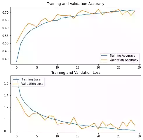

Even though we lost a bit of accuracy there is almost no overfitting thanks to data augmentation.

Summary

This tutorial demonstrated overfitting and underfitting and the commonly used techniques to prevent overfitting in neural networks.

The final code used in this tutorial is available on GitHub in my repository.

You can also directly run the code on Google Colab.

If you have any questions or want to say something, please leave a comment in the section below. Also, don't forget to subscribe to the mailing list to be notified of future posts.