Please consider supporting us by disabling your ad blocker. Thank you for your support.
Please consider supporting us by disabling your ad blocker.
YOLOv3 Object Detection with Deep Learning, OpenCV, and Python
In this post, I'll show you how to use the YOLO model, and specifically YOLOv3, to detect objects in images and real-time videos using Python and OpenCV.
YOLO (You Only Look Once) is a single-stage object detector, meaning it makes predictions for the bounding boxes and class labels of objects in an image in a single pass through the network.
This makes it fast and efficient for real-time object detection applications but it may not be as accurate as some other object detection algorithms, such as R-CNN (Regional Convolutional Neural Network), which is a two-stage detector that uses a separate region proposal step followed by a CNN for classification.
The key idea behind YOLO is to divide the input image into a grid of cells, with each cell responsible for predicting the bounding boxes and class probabilities for the objects present in that cell.
By the end of this tutorial, you will have a good understanding of how to use YOLOv3 for object detection and will be able to apply it to your own projects.
If you want to learn how to train your own YOLO model, I recommend you check out my new book, Mastering YOLO: Build an Automatic Number Plate Recognition System, which is a comprehensive guide to building your own YOLO model from scratch. From data collection to model training and deployment, this book will help you build your understanding of YOLO from the ground up.
Object Detection with YOLOv3 in Images
Now, let's see how to use YOLOv3 with OpenCV.
So that you can follow along with me, here's how I structured the tutorial:
├── examples
│   ├── images
│   │   ├── 1.jpg
│   │   ├── 2.jpg
│   |   └── ...
│   └── videos
│       ├── 1.mp4
│       ├── ...
├── yolov3-config
│   ├── coco.names
│   ├── yolov3.cfg
│   └── yolov3.weights
├── yolov3-images.py
└── yolov3-videos.py
Create a new Python file, name it yolov3_images.py, and copy the following code into it:
import cv2
import numpy as np

# define the minimum confidence (to filter weak detections),
# Non-Maximum Suppression (NMS) threshold, and the green color
confidence_thresh = 0.5
NMS_thresh = 0.3
green = (0, 255, 0)
We start by loading the required libraries. We will be using OpenCV and NumPy. We also define the minimum confidence threshold, the NMS threshold, and the green color.
Here is a brief description of the variables we defined:
-
The confidence_thresh is used to filter out weak detections. In this case, we will use a value of 0.5, which means that only detections with a confidence score above 50% will be kept.
-
The NMS_thresh is used to eliminate overlapping bounding boxes. In our case, we will use a value of 0.3, which means that if the IoU (Intersection over Union) between two bounding boxes is above 30%, the bounding box with the lower confidence score will be discarded.
-
The green variable represents the green color that we will use to draw the bounding boxes on the input image.
Let's now load the input image and the class labels the YOLOv3 model was trained on. Make sure to download the source code for this tutorial to get the class labels file, configuration file, and the images/videos used in this tutorial.
# Load the image and get its dimensions
image = cv2.imread("examples/images/1.jpg")
# resize the image to 25% of its original size
image = cv2.resize(image,
                    (int(image.shape[0] * 0.25),
                     int(image.shape[1] * 0.25)))

# get the image dimensions
h = image.shape[0]
w = image.shape[1]

# load the class labels the model was trained on
classes_path = "yolov3-config/coco.names"
with open(classes_path, "r") as f:
    classes = f.read().strip().split("\n")
Here, we are loading the image and resizing it to 25% of its original size.
We then get the dimensions of the image and load the COCO class labels the YOLOv3 model was trained on.
Next, let's load the weights and configuration file of the YOLOv3 model. You can download the weights file from this link.
# load the configuration and weights from disk
yolo_config = "yolov3-config/yolov3.cfg"
yolo_weights = "yolov3-config/yolov3.weights"

# load YOLOv3 network pre-trained on the COCO dataset
net = cv2.dnn.readNetFromDarknet(yolo_config, yolo_weights)
net.setPreferableBackend(cv2.dnn.DNN_BACKEND_OPENCV)
net.setPreferableTarget(cv2.dnn.DNN_TARGET_CPU)
Here, we are using the readNetFromDarknet function provided by OpenCV to load the YOLOv3 model.
We can also use Pytorch to load the model. If you're interested in learning more about working with Pytorch to load and use YOLO models, be sure to check out my new ebook, Mastering YOLO: Build an Automatic Number Plate Recognition System
We then set the backend and target for the model. In this case, we will use the OpenCV backend and the CPU target. If you have a GPU, you can use the GPU target instead using the following code:
net.setPreferableBackend(cv2.dnn.DNN_BACKEND_CUDA)
net.setPreferableTarget(cv2.dnn.DNN_TARGET_CUDA)
Next, we need to get the output layer names of the model and pass the input image through the network to make predictions.
# Get the name of all the layers in the network
layer_names = net.getLayerNames()
# Get the names of the output layers
output_layers = [layer_names[i[0] - 1] for i in net.getUnconnectedOutLayers()]

# create a blob from the image
blob = cv2.dnn.blobFromImage(
    image, 1 / 255, (416, 416), swapRB=True, crop=False)
# pass the blob through the network and get the output predictions
net.setInput(blob)
outputs = net.forward(output_layers)
Here is a brief description of the code above:
-
We first get the names of all the layers in the network using the getLayerNames function.
-
We then determine the output layer names using the getUnconnectedOutLayers function.
-
Construct a blob from the image using the cv2.dnn.blobFromImage function.
-
Finally, we set the input blob for the network and run the forward pass to get the output predictions.
If you print the output_layers variable, you will see the names of the output layers:
print(output_layers)

['yolo_82', 'yolo_94', 'yolo_106']
The output of the model is a list containing three NumPy arrays. Each array contains the bounding boxes, confidence scores, and class probabilities for each cell in the input image.
print(len(outputs))
print(outputs[0].shape)
print(outputs[1].shape)
print(outputs[2].shape)

3
(507, 85)
(2028, 85)
(8112, 85)
If we look at the first array, we can see that it has a shape of (507, 85).
So there are 507 bounding boxes in the image and each bounding box has 85 values, which are the bounding box coordinates (center_x, center_y, w, h), confidence score, and class probabilities (80 classes).
So now we can loop over the outputs list and extract the bounding boxes, class probabilities, and class IDs. We can then use non-maximum suppression to eliminate the overlapping bounding boxes and select the most confident ones.
# create empty lists for storing the bounding boxes, confidences, and class IDs
boxes = []
confidences = []
class_ids = []

# loop over the output predictions
for output in outputs:
    # loop over the detections
    for detection in output:
        # get the class ID and confidence of the dected object
        scores = detection[5:]
        class_id = np.argmax(scores)
        confidence  = scores[class_id]

        # we keep the bounding boxes if the confidence (i.e. class probability)
        # is greater than the minimum confidence
        if confidence > confidence_thresh:
            # perform element-wise multiplication to get
            # the coordinates of the bounding box
            box = [int(a * b) for a, b in zip(detection[0:4], [w, h, w, h])]
            center_x, center_y, width, height = box

            # get the top-left corner of the bounding box
            x = int(center_x - (width / 2))
            y = int(center_y - (height / 2))

            # append the bounding box, confidence, and class ID to their respective lists
            class_ids.append(class_id)
            confidences.append(float(confidence))
            boxes.append([x, y, width, height])
Here is what we are doing in the above code:
-
We first initialize 3 empty lists for storing the bounding boxes, confidences (class probabilities), and class IDs of the detected objects.
-
We then loop over the output predictions and loop over the detections in each output.
-
For each detection, we get the class ID and confidence (class probability) of the detected object. We then check if the confidence is greater than the minimum confidence threshold. If so, we perform element-wise multiplication to get the coordinates of the bounding box. We then append the class ID, confidence, and bounding box to their respective lists.
YOLO returns bounding boxes in the form of (center_x, center_y, width, height), where (center_x, center_y) is the center of the bounding box, and (width, height) is the width and height of the bounding box.
We need to convert these coordinates to the top-left corner of the bounding box (x, y). This is what we are doing in the above code:
x = int(center_x - (width / 2))
y = int(center_y - (height / 2))
This ensures that the bounding box is properly positioned and aligned with the object in the image.
Let's try to draw the bounding boxes on the input image:
# draw the bounding boxes on a copy of the original image
# before applying non-maxima suppression
image_copy = image.copy()
for box in boxes:
    x, y, width, height = box
    cv2.rectangle(image_copy, (x, y), (x + width, y + height), green, 2)

# show the output image
cv2.imshow("Before NMS", image_copy)
cv2.waitKey(0)
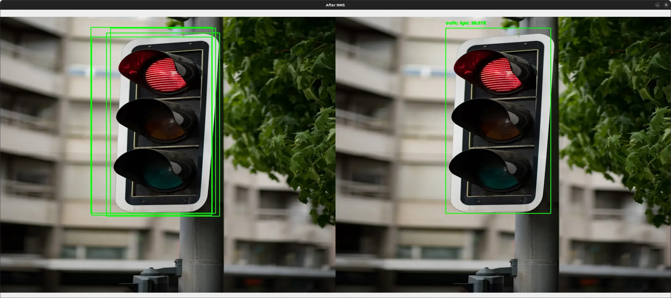
Here is the output image:
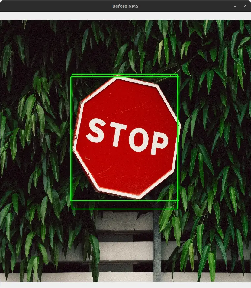
As you can see, there are two bounding boxes around the stop sign. We can use non-maximum suppression (NMS) to eliminate the weaker bounding box and keep only the stronger one.
To apply NMS, we first need to define a confidence threshold and an NMS threshold. The confidence threshold is used to filter out weak detections, and the NMS threshold is used to determine how close two bounding boxes need to be in order to be considered overlapping.
OpenCV provides the cv2.dnn.NMSBoxes function to apply NMS to the bounding boxes.
This function takes 4 arguments: the list of bounding boxes, the list of confidences, the confidence threshold, and the NMS threshold. It returns the indices of the bounding boxes that should be kept after NMS.
# apply non-maximum suppression to remove weak bounding boxes that overlap with others.
indices = cv2.dnn.NMSBoxes(boxes, confidences, confidence_thresh, NMS_thresh)
indices = indices.flatten()
for i in indices:
    (x, y, w, h) = boxes[i][0], boxes[i][1], boxes[i][2], boxes[i][3]
    cv2.rectangle(image, (x, y), (x + w, y + h), green, 2)
    text = f"{classes[class_ids[i]]}: {confidences[i] * 100:.2f}%"
    cv2.putText(image, text, (x, y - 15), cv2.FONT_HERSHEY_SIMPLEX, 0.5, green, 2)

# show the output image
cv2.imshow("After NMS", image)
cv2.waitKey(0)
We loop over the indices and filter the bounding boxes, confidences, and class ID lists using the indices. We then draw the bounding boxes, class labels, and confidences on the input image.
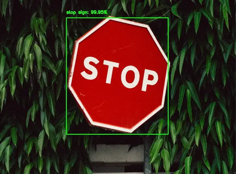
Here is our final result:
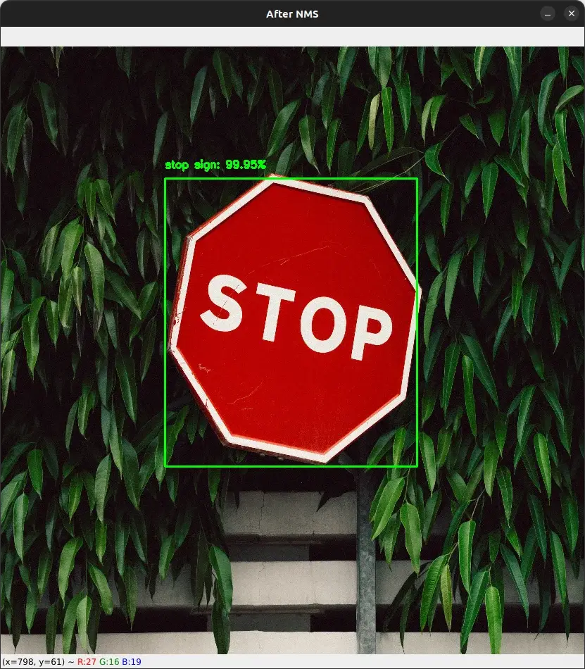
After applying NMS, we can see that there is only one bounding box around the stop sign with a confidence of 99.95%.
Let's try with another image:
You can get the complete code for this tutorial along with the images from this link.
Object Detection with YOLOv3 in Real-Time Video
Now that we have seen how to perform object detection with YOLOv3 in images, let's try to detect objects in real-time video.
The code for this section is almost the same as the code for object detection in images. The only difference is that we need to loop over the frames in the video stream and apply the object detection algorithm to each frame.
import numpy as np
import cv2
import os
import time


# define the minimum confidence (to filter weak detections),
# Non-Maximum Suppression (NMS) threshold, and the green color
confidence_thresh = 0.5
NMS_thresh = 0.3
green = (0, 255, 0)

# Initialize the video capture object
video_cap = cv2.VideoCapture("examples/videos/1.mp4")

# load the class labels the model was trained on
classes_path = "yolov3-config/coco.names"
with open(classes_path, "r") as f:
    classes = f.read().strip().split("\n")

# load the configuration and weights from disk
yolo_config = "yolov3-config/yolov3.cfg"
yolo_weights = "yolov3-config/yolov3.weights"

# load the pre-trained YOLOv3 network
net = cv2.dnn.readNetFromDarknet(yolo_config, yolo_weights)
net.setPreferableBackend(cv2.dnn.DNN_BACKEND_OPENCV)
net.setPreferableTarget(cv2.dnn.DNN_TARGET_CPU)

# Get the name of all the layers in the network
layer_names = net.getLayerNames()
# Get the names of the output layers
output_layers = [layer_names[i[0] - 1] for i in net.getUnconnectedOutLayers()]
The code above is similar to the code for object detection in images. This time, we are importing the time module to calculate the FPS (frames per second) of the video stream.
We are also initializing the video capture object taking advantage of the cv2.VideoCapture class.
Let's now loop over the frames in the video stream and apply the YOLOv3 algorithm to each frame:
while True:
    # start time to compute the fps
    start = time.time()
    # read the video frame
    success, frame = video_cap.read()

    # if there are no more frames to show, break the loop
    if not success:
        break

    # # get the frame dimensions
    h = frame.shape[0]
    w = frame.shape[1]

    # create a blob from the frame
    blob = cv2.dnn.blobFromImage(
        frame, 1 / 255, (416, 416), swapRB=True, crop=False)
    # pass the blog through the network and get the output predictions
    net.setInput(blob)
    outputs = net.forward(output_layers)

    # create empty lists for storing the bounding boxes, confidences, and class IDs
    boxes = []
    confidences = []
    class_ids = []

    # loop over the output predictions
    for output in outputs:
        # loop over the detections
        for detection in output:
            # get the class ID and confidence of the dected object
            scores = detection[5:]
            class_id = np.argmax(scores)
            confidence  = scores[class_id]

            # filter out weak detections by keeping only those with a confidence
            # above the minimum confidence threshold (0.5 in this case).
            if confidence > confidence_thresh:
                # perform element-wise multiplication to get
                # the coordinates of the bounding box
                box = [int(a * b) for a, b in zip(detection[0:4], [w, h, w, h])]
                center_x, center_y, width, height = box

                # get the top-left corner of the bounding box
                x = int(center_x - (width / 2))
                y = int(center_y - (height / 2))

                # append the bounding box, confidence, and class ID to their respective lists
                class_ids.append(class_id)
                confidences.append(float(confidence))
                boxes.append([x, y, width, height])
First, we are reading the frames from the video stream using video_cap.read() and loop over them until there are no more frames to show.
For each frame, we create a blob and pass it through the YOLOv3 network to get the output predictions.
Then, we loop over the output predictions and loop over the detections. For each detection, we get the bounding boxes, class ID, and confidence of the detected object and store them in their respective lists.
Finally, we can apply non-maxima suppression to the bounding boxes to remove overlapping bounding boxes:
    # apply non-maximum suppression to remove weak bounding boxes that overlap with others.
    indices = cv2.dnn.NMSBoxes(boxes, confidences, confidence_thresh, NMS_thresh)
    indices = indices.flatten()

    for i in indices:
        (x, y, w, h) = boxes[i][0], boxes[i][1], boxes[i][2], boxes[i][3]
        cv2.rectangle(frame, (x, y), (x + w, y + h), green, 2)
        text = f"{classes[class_ids[i]]}: {confidences[i] * 100:.2f}%"
        cv2.putText(frame, text, (x, y - 5), cv2.FONT_HERSHEY_SIMPLEX, 0.5, green, 2)

    # end time to compute the fps
    end = time.time()
    # calculate the frame per second and draw it on the frame
    fps = f"FPS: {1 / (end - start):.2f}"
    cv2.putText(frame, fps, (50, 50),
                cv2.FONT_HERSHEY_SIMPLEX, 2, (0, 0, 255), 8)

    # display the frame
    cv2.imshow("Frame", frame)
    # if the 'q' key is pressed, stop the loop
    if cv2.waitKey(30) == ord("q"):
        break

# release the video capture object
video_cap.release()
cv2.destroyAllWindows()
After applying non-maxima suppression, we loop over the indices and draw the bounding boxes, confidences, and class labels on the frame.
Finally, we calculate the FPS of the video stream and display the frame.
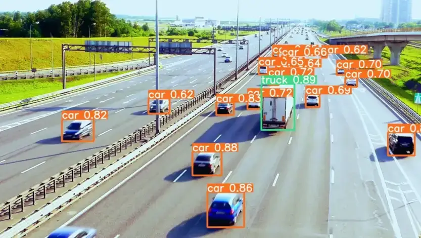
The video below shows the output of the code above:
We can see that the cars are detected with high accuracy. However, the FPS is not very high (around 4 FPS). This is because we are using the CPU to perform the detection. If we use a GPU, we can get a higher FPS.
But for that, we need to install the CUDA toolkit, cuDNN, and compile OpenCV with CUDA support. To learn how to Install CUDA and cuDNN for GPU support, check out my book, Mastering YOLO: Build an Automatic Number Plate Recognition System where I provide a detailed guide that covers every step in the process.
Summary
In this tutorial, we learned how to perform object detection in images and videos using YOLOv3 with OpenCV and Python.
I also showed you how to apply non-maxima suppression to remove overlapping bounding boxes.
The code for this tutorial is available from this link.
Related Tutorials
Here are some related tutorials that you may find interesting:
Previous Article
Object Detection with YOLO using PyTorch
Next Article