Transfer Learning with Keras, TensorFlow, and Python

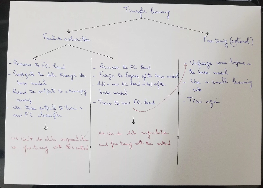
I mentioned in the previous tutorial that there are two ways to do transfer learning via feature extraction:

• Remove the head of the base model.
• Propagate the training data through the base model.
• Record the outputs to a Numpy array, CSV file, or something else.
• Use these outputs to train a new classifier.

Or we can use feature extraction like this:

• Remove the head from the base model.
• Add a new classifier on top of the base model.
• Freeze the layers of the base model.
• Train the new classifier.

We already saw in the previous tutorial how to do transfer learning with the second option. So in today's blog post, I will show you how to do transfer learning via feature extraction with the first option to classify images of flowers.

We will be using the VGG16 pre-trained model as our base model for feature extraction.

I made a small diagram by hand to help you get an overall idea if you are feeling a little lost, it's not the best diagram in the world but it can help x) (let me know what you think):

Let's not waste our time and get started.

Import Libraries and Download the Dataset

from tensorflow.keras import Sequential
from tensorflow.keras import layers
import tensorflow_datasets as tfds
from tensorflow import keras
import tensorflow as tf
import matplotlib.pyplot as plt
import numpy as np

We are going to use TensorFlow Datasets to load the dataset:

ds, info = tfds.load('tf_flowers',
              # take 80% for training, 10% for validation, and 10% for testing
              split=["train[:80%]", "train[80%:90%]", "train[90%:100%]"],
              as_supervised=True,
              with_info=True)
train_set, valid_set, test_set = ds

The dataset contains 3670 images of flowers and there are 5 classes:

info.splits['train'].num_examples
>>> 3670
class_names = info.features['label'].names
class_names
>>> ['dandelion', 'daisy', 'tulips', 'sunflowers', 'roses']

Visualize the Images

let's visualize some images from the dataset:

plt.figure(figsize=(10, 10))
i = 0
for image, label in train_set.take(9):
    plt.subplot(3, 3, i + 1)
    image = tf.image.resize(image, (224, 224))
    plt.imshow(image.numpy().astype("uint8"))
    plt.title(class_names[label])
    plt.axis("off")
    i += 1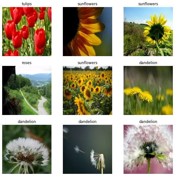

Prepare the Dataset

Next, we need to preprocess our images. We first need to resize them to 224 x 224 pixels and standardize the pixel values to the [0, 1] range. We will also shuffle the training set and batch and prefetch all the datasets.

Let's create a simple function for that:

# declare some variables
batch_size = 32
img_height = 224
img_width = 224
AUTOTUNE = tf.data.AUTOTUNE

# We will use this layer to standardize the pixel values
rescaling_layer = layers.Rescaling(1./255)


def create_dataset(ds, shuffle=False):
    if shuffle:
        ds = ds.shuffle(1000)
    # resize the images
    ds = ds.map(
        lambda x, y: (tf.image.resize(x, (img_height, img_width)), y)
    )
    # standardize the pixel values to the [0 ,1] range
    ds = ds.map(lambda x, y: (rescaling_layer(x), y))
    ds = ds.batch(batch_size)
    ds = ds.prefetch(AUTOTUNE)
    return ds

train_set = create_dataset(train_set, shuffle=True)
valid_set = create_dataset(valid_set)
test_set = create_dataset(test_set)

Extract the Features

Let's first start by loading the VGG16 model:

from keras.applications.vgg16 import VGG16

img_size = (img_height, img_width, 3)
conv_base = VGG16(input_shape=(img_size),
                   include_top=False,
                   weights='imagenet')

Here is the architecture of the VGG16:

Model: "vgg16"
_________________________________________________________________
Layer (type)                 Output Shape              Param #   
=================================================================
input_1 (InputLayer)         [(None, 224, 224, 3)]     0         
_________________________________________________________________
block1_conv1 (Conv2D)        (None, 224, 224, 64)      1792      
_________________________________________________________________
block1_conv2 (Conv2D)        (None, 224, 224, 64)      36928     
_________________________________________________________________
block1_pool (MaxPooling2D)   (None, 112, 112, 64)      0         
_________________________________________________________________
block2_conv1 (Conv2D)        (None, 112, 112, 128)     73856     
_________________________________________________________________
block2_conv2 (Conv2D)        (None, 112, 112, 128)     147584    
_________________________________________________________________
block2_pool (MaxPooling2D)   (None, 56, 56, 128)       0         
_________________________________________________________________
block3_conv1 (Conv2D)        (None, 56, 56, 256)       295168    
_________________________________________________________________
block3_conv2 (Conv2D)        (None, 56, 56, 256)       590080    
_________________________________________________________________
block3_conv3 (Conv2D)        (None, 56, 56, 256)       590080    
_________________________________________________________________
block3_pool (MaxPooling2D)   (None, 28, 28, 256)       0         
_________________________________________________________________
block4_conv1 (Conv2D)        (None, 28, 28, 512)       1180160   
_________________________________________________________________
block4_conv2 (Conv2D)        (None, 28, 28, 512)       2359808   
_________________________________________________________________
block4_conv3 (Conv2D)        (None, 28, 28, 512)       2359808   
_________________________________________________________________
block4_pool (MaxPooling2D)   (None, 14, 14, 512)       0         
_________________________________________________________________
block5_conv1 (Conv2D)        (None, 14, 14, 512)       2359808   
_________________________________________________________________
block5_conv2 (Conv2D)        (None, 14, 14, 512)       2359808   
_________________________________________________________________
block5_conv3 (Conv2D)        (None, 14, 14, 512)       2359808   
_________________________________________________________________
block5_pool (MaxPooling2D)   (None, 7, 7, 512)         0         
=================================================================
Total params: 14,714,688
Trainable params: 14,714,688
Non-trainable params: 0
_________________________________________________________________

The last layer has a shape of (7, 7, 512) so this will be the shape of the extracted features. We will use these features to train a new FC classifier so we need to flatten them before feeding them to the FC classifier.

Let's create a helper function to extract those features as well as their labels. 

def extract_features(dataset):
    # here we will store the extracted features and their labels
    features = []
    labels = []

    total_batches = tf.data.experimental.cardinality(dataset)
    current_batch = 1

    # loop over the dataset to get batches of images and their labels
    for images_batch, labels_batch in dataset:
        print("[INFO] processing batch {}/{}".format(current_batch, total_batches))
        # extract the features using the predict method
        # the shape will be (32, 7, 7, 512)
        features_batch = conv_base.predict(images_batch)

        # store the current batch of features and labels in a list
        features.append(features_batch)
        labels.append(labels_batch)
        current_batch += 1

    features = np.vstack(features) # shape: (2936, 7, 7, 512)
    labels = np.hstack(labels)     # shape: (2936,)
    # flatten the features
    features = features.reshape(features.shape[0], 7 * 7 * 512)

    return features, labels


print('[INFO] extracting features from training dataset ...')
train_features, train_labels = extract_features(train_set)
print('[INFO] extracting features from validation dataset ...')
validation_features, validation_labels = extract_features(valid_set)

output:

[INFO] extracting features from training dataset ...
[INFO] processing batch 1/92
[INFO] processing batch 2/92
[INFO] processing batch 3/92
[INFO] processing batch 4/92
[INFO] processing batch 5/92
...
[INFO] extracting features from validation dataset ...
[INFO] processing batch 1/12
[INFO] processing batch 2/12
[INFO] processing batch 3/12
[INFO] processing batch 4/12
[INFO] processing batch 5/12
...

we start by looping over the dataset to get batches of images (each batch is of shape (32, 224, 224, 3)) and their labels.

Then we pass the batch of images through the network to extract a batch of features using the predict method (each batch is of shape (32, 7, 7, 512)).

After each iteration, we append each batch of features and labels to the features and labels lists respectively.

In the case of the training set, after finishing looping over the dataset, the features list will contain 92 batches of shape (32, 7, 7, 512). So we used Numpy to stack these batches vertically; this will give us a shape of (2936, 7, 7, 512).

We finally reshape the features array into a feature vector of shape (2936, 7 x 7 x 512). This is necessary because we are going to feed these features into a densely connected classifier.

Train a New FC Classifier on the Extracted Features

Now we are ready to define a densely connected classifier and train it on the features and labels we have above:

model = Sequential([
    layers.Dense(128, activation='relu', input_dim=7 * 7 * 512),
    layers.Dense(5, activation='softmax')
])

model.compile(optimizer='adam',
              loss='sparse_categorical_crossentropy',
              metrics=['accuracy'])

history = model.fit(train_features, train_labels,
                    epochs=10,
                    validation_data=(validation_features, validation_labels))

Epoch 1/10
92/92 [==============================] - 1s 6ms/step - loss: 1.0842 - accuracy: 0.6655 - val_loss: 0.5425 - val_accuracy: 0.8147
Epoch 2/10
92/92 [==============================] - 0s 4ms/step - loss: 0.3790 - accuracy: 0.8719 - val_loss: 0.5353 - val_accuracy: 0.8229
...
Epoch 9/10
92/92 [==============================] - 0s 4ms/step - loss: 0.0138 - accuracy: 0.9997 - val_loss: 0.5863 - val_accuracy: 0.8174
Epoch 10/10
92/92 [==============================] - 0s 4ms/step - loss: 0.0086 - accuracy: 0.9997 - val_loss: 0.5607 - val_accuracy: 0.8392

Visualize the Results

Let's plot the loss and the accuracy curves on the training and validation sets:

def plot_learning_curves():
    acc = history.history['accuracy']
    val_acc = history.history['val_accuracy']

    loss = history.history['loss']
    val_loss = history.history['val_loss']

    plt.figure(figsize=(10, 8))
    plt.subplot(2, 1, 1)
    plt.plot(acc, label="Training Accuracy")
    plt.plot(val_acc, label="Validation Accuracy")
    plt.legend()
    plt.grid(True)

    plt.subplot(2, 1, 2)
    plt.plot(loss, label="Training Loss")
    plt.plot(val_loss, label="Validation Loss")
    plt.legend()
    plt.grid(True)

    plt.show()

plot_learning_curves()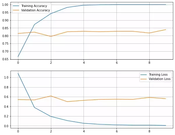

We reached an accuracy of around 83% on the validation set. But because we are not using data augmentation, we can see that the model starts overfitting from almost the beginning.

Transfer Learning with Data Augmentation

I will include an example of transfer learning with data augmentation so that you can compare it with the technique we used above. I will not comment on the code since I have already done a detailed tutorial on transfer learning with data augmentation and fine-tuning.

data_augmentation = Sequential([
    layers.RandomFlip("horizontal", input_shape=(img_size)),
    layers.RandomRotation(0.2),
    layers.RandomZoom(0.2),
  ])

base_model = tf.keras.applications.VGG16(
        input_shape=img_size,
        include_top=False,
        weights="imagenet",
)
# freeze all layers of the base model
base_model.trainable = False

model = Sequential([
    data_augmentation,
    base_model,
    layers.Dropout(0.5),
    layers.Flatten(),
    layers.Dense(128, activation='relu'),
    layers.Dense(5)
])

model.compile(optimizer='adam',
              loss=tf.keras.losses.SparseCategoricalCrossentropy(from_logits=True),
              metrics=['accuracy'])

epochs=10
history = model.fit(
  train_set,
  validation_data=valid_set,
  epochs=epochs
)

output: 

Epoch 1/10
92/92 [==============================] - 8s 74ms/step - loss: 1.3147 - accuracy: 0.5725 - val_loss: 0.6780 - val_accuracy: 0.7602
Epoch 2/10
92/92 [==============================] - 7s 72ms/step - loss: 0.6780 - accuracy: 0.7524 - val_loss: 0.6181 - val_accuracy: 0.7820
...
Epoch 9/10
92/92 [==============================] - 7s 72ms/step - loss: 0.4485 - accuracy: 0.8294 - val_loss: 0.4897 - val_accuracy: 0.8038
Epoch 10/10
92/92 [==============================] - 7s 72ms/step - loss: 0.4309 - accuracy: 0.8396 - val_loss: 0.4956 - val_accuracy: 0.8202

We reached a validation accuracy of 82%. We lost a bit of accuracy but at least there was no overfitting.

You can now unfreeze some layers from the base model and train the whole network with a small learning rate. Please refer to the previous tutorial to see an example of fine-tuning.

Here is the graph of the learning curves:

plot_learning_curves()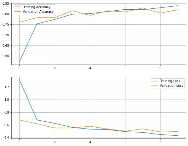

Further Reading

I will leave more resources on the topic if you are looking to go deeper.

Books

This link is an affiliate link, meaning I get a commission if you decide to make a purchase through it, at no cost to you. Thank you for your support!

• Part 2 Chapter 5 from the book Deep Learning with Python.

Articles

• Transfer Learning with Keras and Deep Learning.

Summary

In this tutorial, I showed you how to do transfer learning via feature extraction.

Training with this technique is very fast because the data is only passed into the convolutional base once. But we can't do data augmentation nor fine-tuning with this technique.

The final code used in this tutorial is available on GitHub.

You can also directly run the code on Google Colab or open the notebook on Kaggle.