YOLOv4 Custom Object Detection with OpenCV and Python

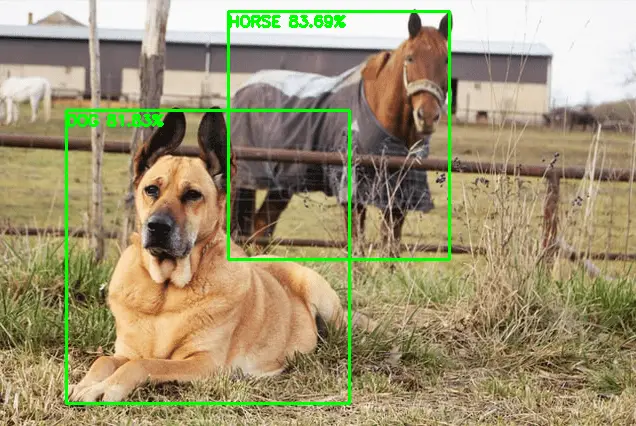
In the previous tutorial, we saw how to use a pre-trained YOLO model to detect objects in images and videos. We learned how to load the weights and configuration files, and how to perform object detection using YOLOv3 and OpenCV.

However, we were limited to detect the classes the pre-trained model was trained on.

In some cases, we may want to detect objects that the model was not trained on. For example, we may want to detect a specific brand of car or a specific type of animal.

In this case, we need to train the model on our custom dataset to detect the objects we want.

In this tutorial, I will show you how to train a YOLOv4 object detector on a custom dataset using OpenCV and Python.

Once our model is trained, we will be able to use it to detect the objects of interest in new images.

We will do this by exporting the trained weights and then creating a separate Python script that loads these weights into the YOLOv4 detector to perform detection of the object of interest.

Training a YOLO model on a custom dataset requires a large amount of data and computational resources. This process can be time-consuming and requires access to a machine with a GPU for efficient training.

To make the process easier and more accessible, I will use Google Colab to train the YOLO detector.

Google Colab provides free access to GPU resources, which will allow us to train the YOLO object detector in a shorter amount of time.

If you're interested in diving deeper into the topic of YOLO and object detection, be sure to check out my new ebook, Mastering YOLO: Build an Automatic Number Plate Recognition System. It's a comprehensive guide to building an end-to-end ANPR system with YOLO, complete with step-by-step tutorials and practical examples.

Our Dataset

The dataset we are going to use in this tutorial is the raccoon dataset from Roboflow.

If you want to get the dataset along with the code for this tutorial, you can download it from here

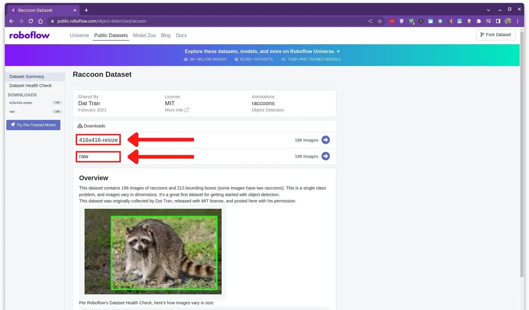
This dataset consists of only 196 images along with their labels that specify the bounding boxes for the raccoons in the images. The dataset is already annotated, so we don't have to do it ourselves.

It is a small and simple dataset that is well-suited for this tutorial, which is to demonstrate the process of training the YOLO detector to detect new objects.

On the home page of the dataset, you can see that there are two versions of the dataset:

• 416x416-resize: This version of the dataset contains resized images of 416x416 pixels. This is the version we will use in this tutorial.
• raw: Images are in their original sizes.

When you click on the 416x416-resize version of the dataset, you will see the following page:

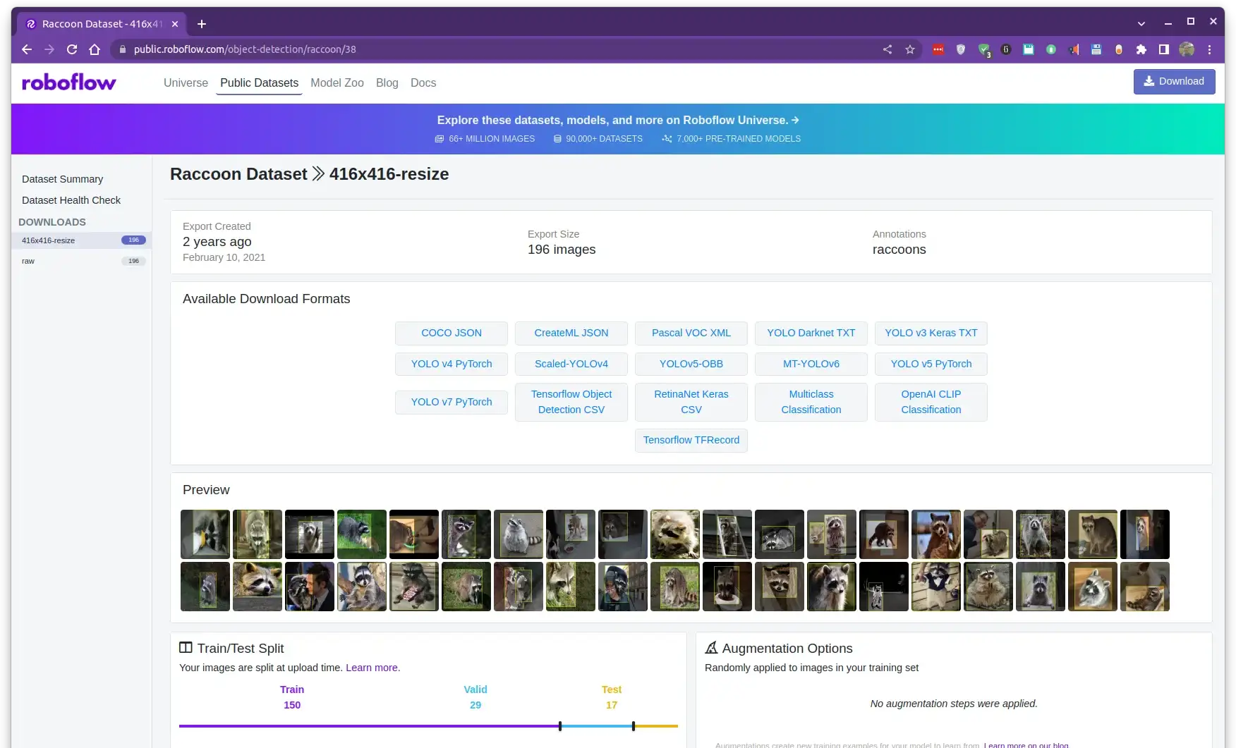
This page contains some information about the dataset, such as the number of images, the training, validation, and test sets. You can also preview some images to get an idea of what the dataset looks like.

Additionally, you can see that there are different available formats for the dataset, including a .tfrecord file, a .coco file, and many other formats that are compatible with different frameworks and models.

You can choose the format based on the model/framework you are using.  In our case, since we are using the YOLOv4 model implemented in the darknet framework, we will download a .darknet file, which is named YOLO Darknet TXT under the Available Download Formats section.

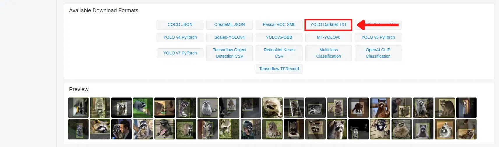
When you click on the YOLO Darknet TXT format, you will be prompted to download the dataset. Click download zip to computer and then on the continue button.

Unzip the downloaded file and you will get the dataset split into training, validation, and test sets:

├── export  [393 entries]
├── README.dataset.txt
├── README.roboflow.txt
├── test  [35 entries]
├── train  [301 entries]
└── valid  [59 entries]

Each of the training, validation, and test sets contains the images and corresponding labels. The labels are stored in a .txt file which contains the bounding box coordinates for the objects in the image along with the class ID for each object (we have only 1 class, so the class ID is always 0).

Since we are going to train the model on Google Colab, we will need to upload our dataset to Google Drive.

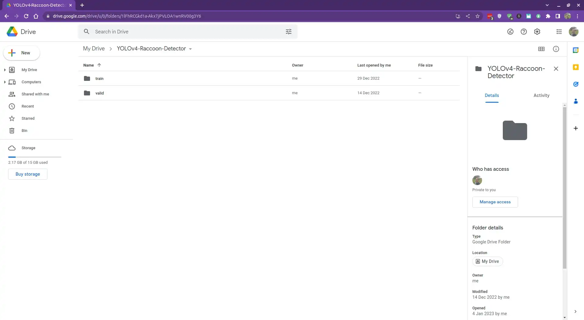
To upload the dataset, first, go to https://drive.google.com and log in to your Google account. Then, create a new folder in your Google Drive and name it YOLOv4-Raccoon-Detector.

Now, upload the dataset to the folder you just created. We just need to upload the train and valid folders; we will use the test set to evaluate our model locally.

Connect to Google Drive

Now that we have uploaded our dataset to Google Drive, we need to connect to Google Drive from Google Colab.

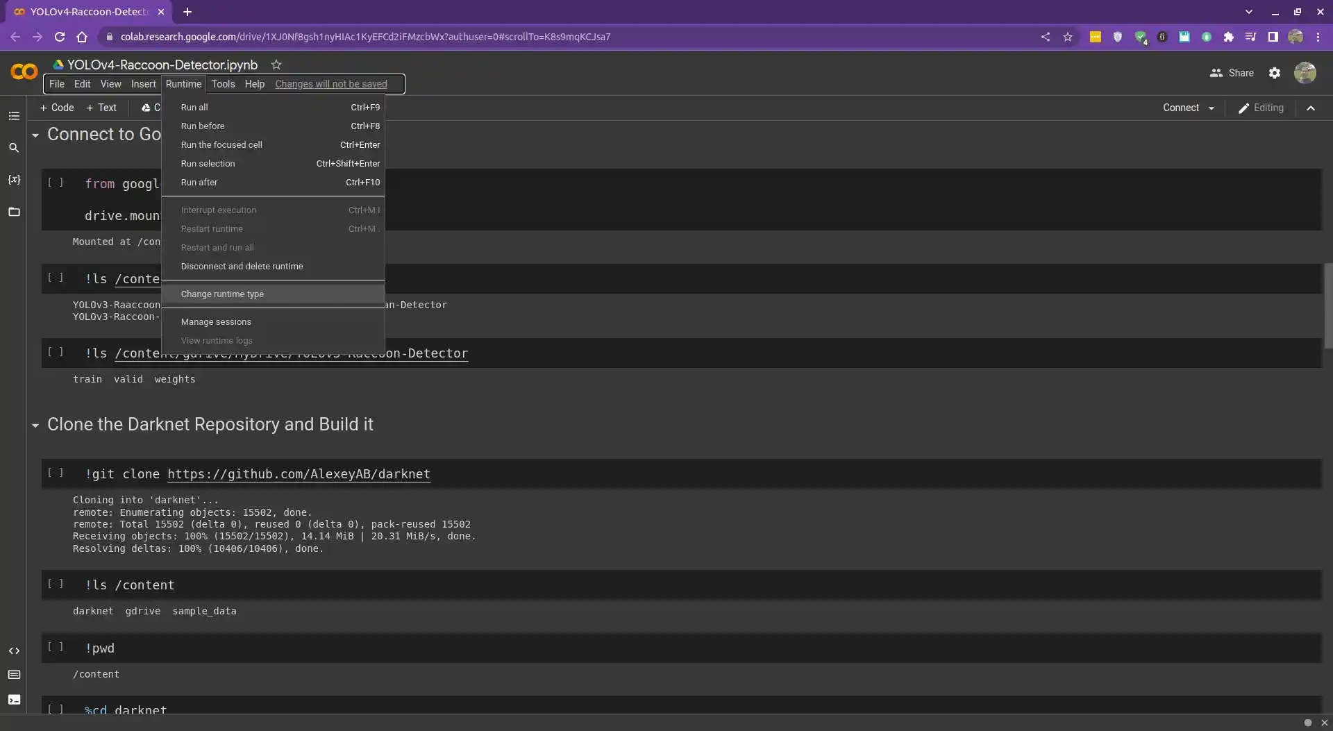
So first, create a new notebook in Google Colab and you can use a GPU instance by clicking on Runtime, then Change runtime type, and then selecting GPU as the hardware accelerator.

Then, run the following code to connect to Google Drive:

from google.colab import drive

drive.mount("/content/gdrive")

Mounted at /content/gdrive

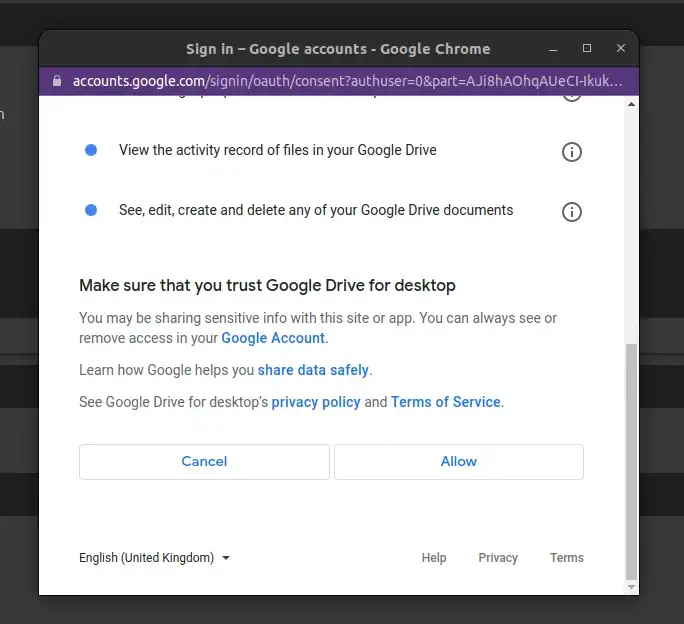
You'll be prompted to permit Google Colab to access your Google Drive.

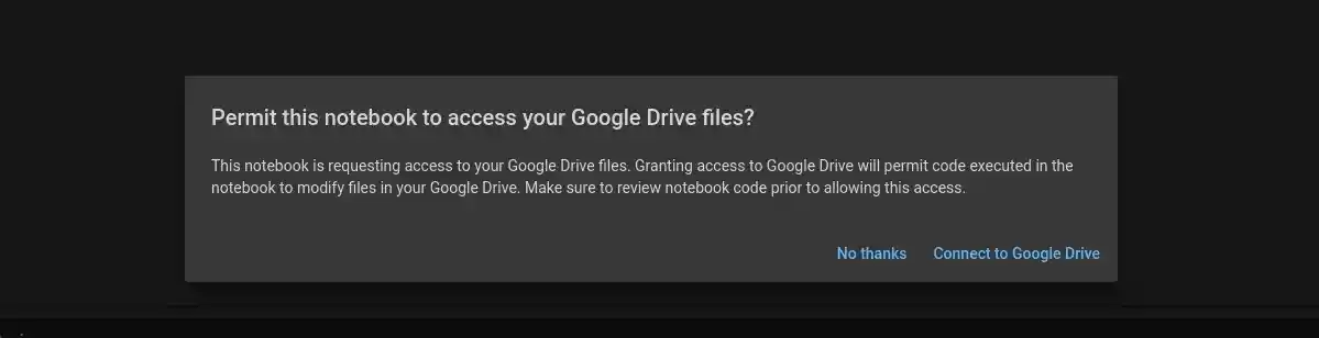
Click Connect to Google Drive, then choose your account, and then click Allow.

From the output of the code above, you can see that Google Drive is mounted at the path content/gdrive.

!ls /content/gdrive/MyDrive

YOLOv4-Raccoon-Detector

!ls /content/gdrive/MyDrive/YOLOv4-Raccoon-Detector

train  valid

Clone the Darknet Repository and Build it

Now that we have connected to Google Drive, we can clone the darknet repository and build it.

Run the following command to clone the Darknet repository:

!git clone https://github.com/AlexeyAB/darknet

Cloning into 'darknet'...
remote: Enumerating objects: 15502, done.
remote: Total 15502 (delta 0), reused 0 (delta 0), pack-reused 15502
Receiving objects: 100% (15502/15502), 14.14 MiB | 20.31 MiB/s, done.
Resolving deltas: 100% (10406/10406), done.

The repository will be cloned in the current directory, which is content.

# print the current directory
!pwd

/content

# list the files in the `content` directory
!ls /content

darknet  gdrive  sample_data

Now, we need to change the directory to darknet and build the darknet repository.

# change the directory to darknet
%cd darknet

!sed -i 's/OPENCV=0/OPENCV=1/' Makefile
!sed -i 's/GPU=0/GPU=1/' Makefile
!sed -i 's/CUDNN=0/CUDNN=1/' Makefile
!make

Here we are using the sed command to change the following lines in the Makefile (which is in the darknet directory):

GPU=1
CUDNN=1
OPENCV=1

The sed command replaces the 0 with 1 in the above lines.

Running the make command will take some time to compile the darknet framework.

After compiling darknet, the next step is to copy the yolov4-tiny-custom.cfg configuration file and make some changes to it.

This file contains information about the model such as the number of layers, the number of filters, the batch size, etc.

!cp cfg/yolov4-tiny-custom.cfg cfg/yolov4-tiny-custom-raccoon.cfg

!sed -i 's/batch=1/batch=64/' cfg/yolov4-tiny-custom-raccoon.cfg
!sed -i 's/subdivisions=1/subdivisions=16/' cfg/yolov4-tiny-custom-raccoon.cfg
!sed -i 's/max_batches = 500200/max_batches = 2000/' cfg/yolov4-tiny-custom-raccoon.cfg
!sed -i 's/steps=400000,450000/steps=1600,1800/' cfg/yolov4-tiny-custom-raccoon.cfg
!sed -i '220 s@classes=80@classes=1@' cfg/yolov4-tiny-custom-raccoon.cfg
!sed -i '269 s@classes=80@classes=1@' cfg/yolov4-tiny-custom-raccoon.cfg
!sed -i '212 s@filters=255@filters=18@' cfg/yolov4-tiny-custom-raccoon.cfg
!sed -i '263 s@filters=255@filters=18@' cfg/yolov4-tiny-custom-raccoon.cfg

Here we copied the yolov4-tiny-custom.cfg, which is in the cfg directory, to yolov4-tiny-custom-raccoon.cfg.

I made these changes as per the instructions in the darknet repository.

In the second line, we changed the batch parameter from 1 to 64. The batch parameter specifies the batch size, which is the number of images that are processed at once during training. So here we are processing 64 images at once during training to update the weights of the model.

The subdivisions parameter determines the number of mini-batches that are used during training. The number of mini-batches is calculated as the batch size divided by the number of subdivisions. For example, if the batch size is 64 and the number of subdivisions is 16, then the model will use 16 mini-batches of size 4 during each iteration of training.

In the third line, we changed the max_batches parameter from 500200 to 2000. This parameter specifies the number of iterations the model will be trained for. A rule of thumb is to set max_batches to 2000 times the number of classes in the dataset (in our case: 2000 * 1 = 2000).

For the classes parameter, we changed the value from 80 to 1 (since we have only one class in our dataset).

Please refer to the darknet repository for more information on the other changes we made to the configuration file.

Download the Pre-trained Weights

We will be using the pre-trained weights yolov4-tiny.conv.29 for the YOLOv4 architecture.

Using pre-trained weights can greatly speed up the training process and improve the performance of the model. This is because pre-trained weights provide a good starting point for the model, which can then be fine-tuned on the specific dataset and task at hand.

%cd /content/
!wget https://github.com/AlexeyAB/darknet/releases/download/darknet_yolo_v4_pre/yolov4-tiny.conv.29

/content
--2023-01-03 10:47:32--  https://github.com/AlexeyAB/darknet/releases/download/darknet_yolo_v4_pre/yolov4-tiny.conv.29
Resolving github.com (github.com)... 140.82.113.3
Connecting to github.com (github.com)|140.82.113.3|:443... connected.
HTTP request sent, awaiting response... 302 Found
Location: https://objects.githubusercontent.com/github-production-release-asset-2e65be/75388965/28807d00-3ea4-11eb-97b5-4c846ecd1d05?X-Amz-Algorithm=AWS4-HMAC-SHA256&X-Amz-Credential=AKIAIWNJYAX4CSVEH53A%2F20230103%2Fus-east-1%2Fs3%2Faws4_request&X-Amz-Date=20230103T104732Z&X-Amz-Expires=300&X-Amz-Signature=d188e5ad0cd024af98fc9c255ef9a11e87ecea18062d35bea9dc82d2e53317ab&X-Amz-SignedHeaders=host&actor_id=0&key_id=0&repo_id=75388965&response-content-disposition=attachment%3B%20filename%3Dyolov4-tiny.conv.29&response-content-type=application%2Foctet-stream [following]
--2023-01-03 10:47:32--  https://objects.githubusercontent.com/github-production-release-asset-2e65be/75388965/28807d00-3ea4-11eb-97b5-4c846ecd1d05?X-Amz-Algorithm=AWS4-HMAC-SHA256&X-Amz-Credential=AKIAIWNJYAX4CSVEH53A%2F20230103%2Fus-east-1%2Fs3%2Faws4_request&X-Amz-Date=20230103T104732Z&X-Amz-Expires=300&X-Amz-Signature=d188e5ad0cd024af98fc9c255ef9a11e87ecea18062d35bea9dc82d2e53317ab&X-Amz-SignedHeaders=host&actor_id=0&key_id=0&repo_id=75388965&response-content-disposition=attachment%3B%20filename%3Dyolov4-tiny.conv.29&response-content-type=application%2Foctet-stream
Resolving objects.githubusercontent.com (objects.githubusercontent.com)... 185.199.108.133, 185.199.109.133, 185.199.110.133, ...
Connecting to objects.githubusercontent.com (objects.githubusercontent.com)|185.199.108.133|:443... connected.
HTTP request sent, awaiting response... 200 OK
Length: 19789716 (19M) [application/octet-stream]
Saving to: ‘yolov4-tiny.conv.29’

yolov4-tiny.conv.29 100%[===================>]  18.87M  56.8MB/s    in 0.3s    

2023-01-03 10:47:33 (56.8 MB/s) - ‘yolov4-tiny.conv.29’ saved [19789716/19789716]

Copy the Images and Labels from Google Drive to Google Colab

Now, we will copy the images and labels that we downloaded from Google Drive in the previous section.

# create a directory to store the training and validation set
!mkdir train
!mkdir valid

# copy the training and validation set from Google Drive to Google Colab
!cp /content/gdrive/MyDrive/YOLOv4-Raccoon-Detector/train/* /content/train/
!cp /content/gdrive/MyDrive/YOLOv4-Raccoon-Detector/valid/* /content/valid/

Configure Darknet for Training the YOLOv4 Object Detector

In order to train the YOLOv4 object detector, we need to configure the Darknet framework to use our custom dataset.

This involves creating a file that contains the names of the classes in our dataset, as well as a file that specifies the location of the training and validation data, the number of classes, and the location where the trained weights will be saved.

!echo "Raccoon" > classes.names
!echo -e 'classes= 1\ntrain  = /content/train.txt\nvalid  = /content/valid.txt\nnames = /content/classes.names\nbackup = /content/gdrive/MyDrive/YOLOv4-Raccoon-Detector' > darknet.data

Here we created a file called classes.names, which contains the name of the class in our dataset (Raccoon).

We also created a file called darknet.data, which contains the following information:

• classes: The number of classes in the dataset (1 in our case).
• train: The path to a file (which we will create in a moment) that contains the paths to the training images (in our case, the path is: /content/train.txt).
• valid: The path to a file (which we will create in a moment) that contains the paths to the validation images (in our case, the path is: /content/valid.txt).
• classes.names: The directory where the trained weights will be saved. In this case, the directory is /content/gdrive/MyDrive/YOLOv4-Raccoon-Detector.

Again, these instructions are based on the darknet repository.

Now we will create a helper function to create and populate the train.txt and valid.txt files with the paths to the images.

# create a helper function to generate a txt file containing the path to all the images in the dataset
import glob

def generate_txt(root_dir, filename):
  """ 
  Generate a txt file containing the path to the images in the `root_dir` directory
  """
  images_list = glob.glob(root_dir + "*.jpg")

  with open(filename, "w") as f:
    f.write("\n".join(images_list))
  
generate_txt("/content/train/", "train.txt")
generate_txt("/content/valid/", "valid.txt")

This function takes in the path to the directory containing the images and the name of the file to be created. It then creates a txt file containing the path to all the images in the directory.

Now you should see the train.txt and valid.txt files in the file explorer on the left side of the screen.

!apt-get install tree
!tree --filelimit 10

├── classes.names
├── darknet [29 entries]
├── darknet.data
├── gdrive
│   └── MyDrive
│       ├── YOLOv4-Raccoon-Detector
│       │   ├── train [301 entries]
│       │   └── valid [59 entries]
├── sample_data
│   ├── ...
├── train [301 entries]
├── train.txt
├── valid [59 entries]
├── valid.txt
└── yolov4-tiny.conv.29

And here is what the train.txt file contains:

!head train.txt

/content/train/raccoon-13_jpg.rf.0918508bfbd0c037e5be53199af99385.jpg
/content/train/raccoon-187_jpg.rf.5e8387ff3865ebe655fb8b1fd2d6f035.jpg
/content/train/raccoon-18_jpg.rf.7f0002ee716e2f8a7b18f1262db1dda7.jpg
/content/train/raccoon-25_jpg.rf.20ee010f201128760aa1be90e68c9f08.jpg
/content/train/raccoon-146_jpg.rf.4de57fce0a75e7c990fe92c4a00c09b1.jpg
/content/train/raccoon-100_jpg.rf.096570afc98c924339283027a04dff6b.jpg
/content/train/raccoon-154_jpg.rf.4154741b6f2f118f1a5b85e6e3ee7719.jpg
/content/train/raccoon-103_jpg.rf.92825fec6281b091e45cddb75301082d.jpg
/content/train/raccoon-44_jpg.rf.532af23d718f38f371c5710e5da9bb47.jpg
/content/train/raccoon-184_jpg.rf.e68000b992ebe291de26b2cbc08c5e71.jpg

Train the YOLOv4 Object Detector on our Custom Dataset

Now that we have configured Darknet to use our custom dataset, we can proceed to train the YOLOv4 object detector.

For this, we first need to change the directory to the Darknet folder and then run the training command.

%cd darknet
!./darknet detector train /content/darknet.data cfg/yolov4-tiny-custom-raccoon.cfg /content/yolov4-tiny.conv.29 -dont_show > /content/gdrive/MyDrive/YOLOv4-Raccoon-Detector/train.log 

We are using the darknet.data and the yolov4-tiny-custom-raccoon.cfg files we created earlier to train the YOLOv4 object detector.

We are also using the yolov4-tiny.conv.29 file as the pre-trained weights file.

The -dont_show flag tells Darknet not to show the training progress in a window (we will use the train.log file to monitor the training progress).

The training process will take a while. You can monitor the training progress by opening the train.log file, which is being updated in real-time.

!head -n 20 /content/gdrive/MyDrive/YOLOv4-Raccoon-Detector/train.log

yolov4-tiny-custom-raccoon
net.optimized_memory = 0 
mini_batch = 4, batch = 64, time_steps = 1, train = 1 
Create CUDA-stream - 0 
 Create cudnn-handle 0 
nms_kind: greedynms (1), beta = 0.600000 
nms_kind: greedynms (1), beta = 0.600000 

 seen 64, trained: 0 K-images (0 Kilo-batches_64) 
Learning Rate: 0.00261, Momentum: 0.9, Decay: 0.0005
 Detection layer: 30 - type = 28 
 Detection layer: 37 - type = 28 
Loaded: 0.758967 seconds

 1: 358.387360, 358.387360 avg loss, 0.000000 rate, 1.202372 seconds, 64 images, -1.000000 hours left
Loaded: 0.000099 seconds

 2: 358.392365, 358.387848 avg loss, 0.000000 rate, 0.698355 seconds, 128 images, 1.089192 hours left
Loaded: 0.000072 seconds

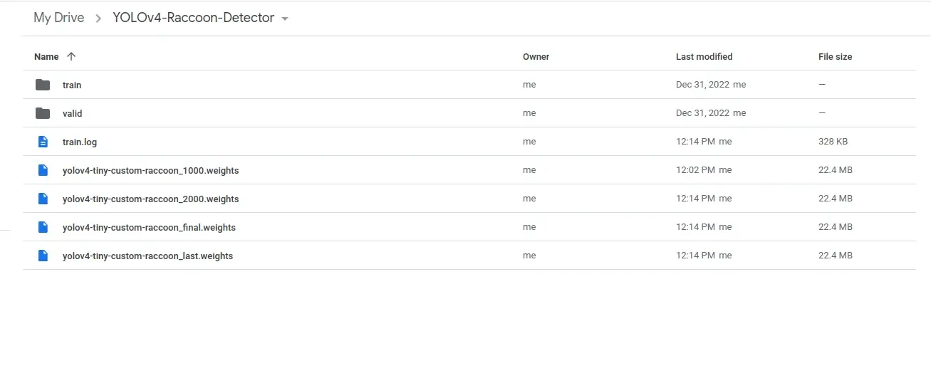
After the training is complete, you should find 4 .weights files in the YOLOv4-Raccoon-Detector folder in Google Drive.

We will use the yolov4-tiny-custom-raccoon_final.weights file for inference.

Create a Python Script to Perform Object Detection

Now that our model is trained, we can use it to perform object detection on new images.

Let's create a Python script, detect.py, to test our model on new images.

You can continue this section in the Colab notebook or you can create a new Python script on your local machine.

In my case, I will create a new Python script on my local machine and download the weights and configuration files from Google Drive (yolov4-tiny-custom-raccoon_final.weights and yolov4-tiny-custom-raccoon.cfg).

Here is how I structured my folder:

tree --filelimit 10

├── detect.py
├── Raccoon
│   ├── export  [393 entries]
│   ├── README.dataset.txt
│   ├── README.roboflow.txt
│   ├── test  [35 entries]
│   ├── train  [301 entries]
│   └── valid  [59 entries]
├── yolov4-tiny-custom-raccoon.cfg
└── yolov4-tiny-custom-raccoon_final.weights

Now, let's write some code:

import cv2
import glob


# define the minimum confidence (to filter weak detections), 
# Non-Maximum Suppression (NMS) threshold, the green color, and the label
confidence_thresh = 0.5
NMS_thresh = 0.3
green = (0, 255, 0)
label = "Raccoon"

We start by loading the required libraries. We will be using OpenCV and the glob module.

We also define the minimum confidence threshold, the NMS threshold, the green color, and the label.

Let's now load the input image. Make sure to download the source code for this tutorial to get the dataset along with all the required files.

# get the list of all the images in the test folder
images_list = glob.glob("Raccoon/test/*.jpg")

for image_path in images_list:
    image = cv2.imread(image_path)

    # get the image dimensions
    h = image.shape[0]
    w = image.shape[1]
        
    # load the configuration and weights files from disk
    yolo_config = "yolov4-tiny-custom-raccoon.cfg"
    yolo_weights = "yolov4-tiny-custom-raccoon_final.weights"

We get the list of all the images in the test folder using the glob module.

We then iterate through the list of image paths and read each image from disk.

Next, we retrieve the height and width of each image and load the configuration and weights files for the YOLOv4 model.

Now, let's load the YOLOv4 model trained on the raccoon dataset:

    # load the YOLOv4 network pre-trained on our raccoon dataset
    net = cv2.dnn.readNetFromDarknet(yolo_config, yolo_weights)

    # Get the name of all the layers in the network
    layer_names = net.getLayerNames()
    # Get the names of the output layers
    output_layers = [layer_names[i[0] - 1] for i in net.getUnconnectedOutLayers()]

    # create a blob from the image
    blob = cv2.dnn.blobFromImage(
        image, 1 / 255, (416, 416), swapRB=True, crop=False)
    # pass the blob through the network and get the output predictions
    net.setInput(blob)
    outputs = net.forward(output_layers)

Here, we are using the readNetFromDarknet function provided by OpenCV to load the YOLO model.

However, we can also use Pytorch to load the model. If you're interested in learning more about working with Pytorch to load and use YOLO models, be sure to check out my new ebook, Mastering YOLO: Build an Automatic Number Plate Recognition System.

Next, we get the names of the layers in the network and then the names of the output layers.

We then create a blob from the image using the cv2.dnn.blobFromImage() function.

Finally, we pass the blob through the network and retrieve the output predictions.

The output predictions contain information about the detected objects in the image, which can be used to draw bounding boxes around the objects and label them with their class.

Let's take a closer look at the output predictions:

print(len(outputs))
print(outputs[0].shape)
print(outputs[1].shape)

2
(507, 6)
(2028, 6)

So here outputs is a list of 2 NumPy arrays. The first array has a shape of (507, 6) and the second array has a shape of (2028, 6).

So, for the first array, there are 507 bounding boxes in the image and each bounding box has 6 values, which are the bounding box coordinates (center_x, center_y, w, h), confidence score (probability that there is an object in the bounding box), and the class probability.

So now we can loop over the outputs list and extract the bounding boxes and the class probability. We can then use non-maximum suppression to eliminate the overlapping bounding boxes and select the most confident ones.

    # create empty lists for storing the bounding boxes and confidences
    boxes = []
    confidences = []

    # loop over the output predictions
    for output in outputs:
        # loop over the detections
        for detection in output:
            # get the confidence of the dected object
            confidence = detection[5]

            # we keep the bounding boxes if the confidence (i.e. class probability) 
            # is greater than the minimum confidence 
            if confidence > confidence_thresh:
                # perform element-wise multiplication to get
                # the coordinates of the bounding box
                box = [int(a * b) for a, b in zip(detection[0:4], [w, h, w, h])]
                center_x, center_y, width, height = box
                
                # get the top-left corner of the bounding box
                x = int(center_x - (width / 2))
                y = int(center_y - (height / 2))

                # append the bounding box and the confidence to their respective lists
                confidences.append(float(confidence))
                boxes.append([x, y, width, height])

We first create empty lists for storing the bounding boxes and the confidences (class probabilities).

We then loop over the output predictions and loop over the detections.

For each detection, we get the confidence (class probability) of the detected object. We then check if the confidence is greater than the minimum confidence threshold.

If so, we perform element-wise multiplication to get the coordinates of the bounding box. We then append the confidence and the bounding box to their respective lists.

The model returns the bounding boxes of the detected objects as a set of coordinates that represent the center of the bounding box and its width and height (center_x, center_y, width, height).

To display the bounding box on the image, we need to convert these coordinates to the top-left corner of the bounding box. This is done in the code above by subtracting half the width and height from the center coordinates.

The final step is to apply non-maximum suppression to eliminate the overlapping bounding boxes and select the most confident ones.

    # apply non-maximum suppression to remove weak bounding boxes that overlap with others.
    indices = cv2.dnn.NMSBoxes(boxes, confidences, confidence_thresh, NMS_thresh)
    
    # loop over the indices only if the `indices` list is not empty
    if len(indices) > 0:
        # loop over the indices
        for i in indices.flatten():
            (x, y, w, h) = boxes[i][0], boxes[i][1], boxes[i][2], boxes[i][3]
            cv2.rectangle(image, (x, y), (x + w, y + h), green, 2)
            text = f"{label}: {confidences[i] * 100:.2f}%"
            cv2.putText(image, text, (x, y - 15), cv2.FONT_HERSHEY_SIMPLEX, 0.5, green, 2)

    # show the output image
    cv2.imshow("Image", image)
    cv2.waitKey(0)

Non-maximum suppression is used in object detection to eliminate overlapping bounding boxes that correspond to the same object.

For that, we can use the cv2.dnn.NMSBoxes function, which takes in a list of bounding boxes, a list of confidence scores, and two threshold values: confidence_thresh and NMS_thresh.

The function returns a list of indices for the bounding boxes that pass the threshold.

If the list of indices is not empty, we loop over the indices and draw the bounding boxes on the image using the cv2.rectangle function.

We finally label the bounding box with the class name, write the confidence score, and display the image.

The screenshot below shows the output of several test images.

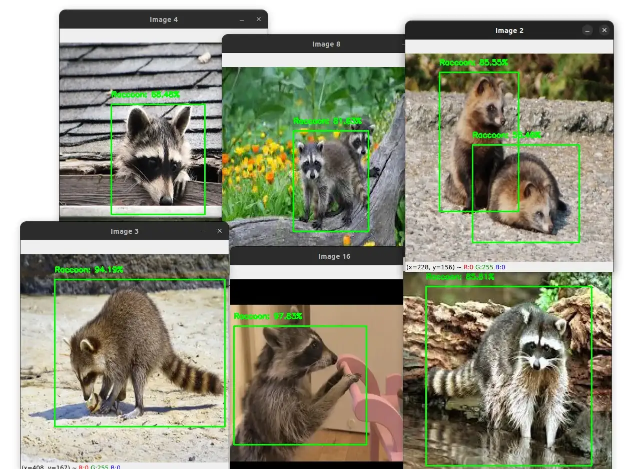
As you can see, the model is able to detect the raccoons in all these images with a high confidence score.

Conclusion

In this tutorial, we learned how to train a custom object detector using the YOLOv4 model.

The steps you need to follow to train a custom object detector are:

1. Get the dataset (In our case, we get it from Roboflow).

2. Annotate the dataset (in our case, the dataset was already annotated).

3. Clone the darknet repository.

4. Edit the Makefile to enable GPU, CUDNN, and OPENCV.

5. Run the make command to build darknet.

6. Copy the .cfg file and make changes to it.

7. Download the weights file.

8. Configure darknet for training the model.

9. Train the model.

10. Export the weights file.

11. Write a Python script to load the model and perform inference.

You can experiment with the model by changing the hyperparameters and the number of training iterations and train the model on a different dataset.

I hope you found this tutorial useful. If you have any questions, feel free to leave a comment below.

While this tutorial provides a great introduction to training custom object detection models with YOLOv4, my new ebook Mastering YOLO: Build an Automatic Number Plate Recognition System takes things to the next level.

In the book, we'll use a PyTorch implementation of YOLO instead of Darknet, and we'll create our own custom dataset by collecting images ourselves and annotating them with an annotation tool. This approach will give you more control over the data. Plus, with step-by-step tutorials and practical examples, you'll gain hands-on coding experience and real-world implementation skills that you can apply to your own projects.

To learn more, click here.

The code for this tutorial is available here

Related Tutorials

You might be interested in the following tutorials:

1. Object Detection with Python, Deep Learning, and OpenCV

2. Object Detection with YOLO using PyTorch

3. YOLOv3 Object Detection with Deep Learning, OpenCV, and Python