Please consider supporting us by disabling your ad blocker. Thank you for your support.
Please consider supporting us by disabling your ad blocker.
Image Filtering and Blurring with OpenCV and Python
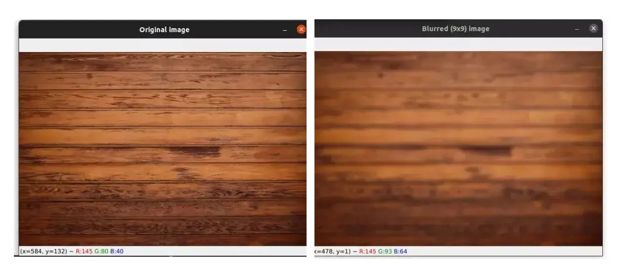
Image blurring is an important preprocessing step in computer vision. It is used to reduce noise and unnecessary detail in an image.
In this tutorial, we will cover four blurring techniques:
- Average blurring using cv2.blur.
- Gaussian blurring using cv2.GaussianBlur.
- Median blurring using cv2.medianBlur.
- Bilateral blurring using cv2.bilateralFilter.
This article is part 8 of the tutorial series on computer vision and image processing with OpenCV:
- How to Read, Write, and Save Images with OpenCV and Python
- How to Read and Write Videos with OpenCV and Python
- How to Resize Images with OpenCV and Python
- How to Crop Images with OpenCV and Python
- How to Rotate Images with OpenCV and Python
- How to Annotate Images with OpenCV and Python (coming soon)
- Bitwise Operations and Image Masking with OpenCV and Python (coming soon)
- Image Filtering and Blurring with OpenCV and Python (this article)
- Image Thresholding with OpenCV and Python
- Morphological Operations with OpenCV and Python
- Edge and Contour Detection with OpenCV and Python
The image below will be used throughout this part:


Average Blurring
Blurring an image means convolving the image with an MxN matrix called a filter or a kernel. Both M and N need to be odd (e.g. 3×3, 5×5, 9×9, etc.).
Since we want to apply average blurring, the kernel needs to be normalized. Here is an example of a 3x3 normalized kernel:
So to blur our image, we take the kernel and slide it over the image from left-to-right and from top-to-bottom and multiply each element in the kernel with each element in the input image region, then sum the result of those multiplications into a single value.
Put simply, we take the sum of the element-wise multiplication with the input image region and the kernel.
This new "averaged" value will replace the value of the pixel located at the center of the kernel. We do this operation for each and every pixel in our input image.
Let's write some code to see how blurring works:
import cv2

image = cv2.imread("wood.jpg")
cv2.imshow("Original image", image)

blurred_3x3 = cv2.blur(image, (3, 3))
cv2.imshow("Blurred (3x3) image", blurred_3x3)

blurred_9x9 = cv2.blur(image, (9, 9))
cv2.imshow("Blurred (9x9) image", blurred_9x9)

cv2.waitKey(0)
We start by loading our image from disk and displaying it.
Then we used the cv2.blur function to apply average blurring to our image. This function takes an image as a first argument and the kernel size as a second argument.
In the first example, we used a kernel size of 3x3, and in the second example, we used a kernel size of 9x9.
Increasing the size of the kernel will result in a more blurry image.
Take a look at the image below to see the result of the cv2.blur function:
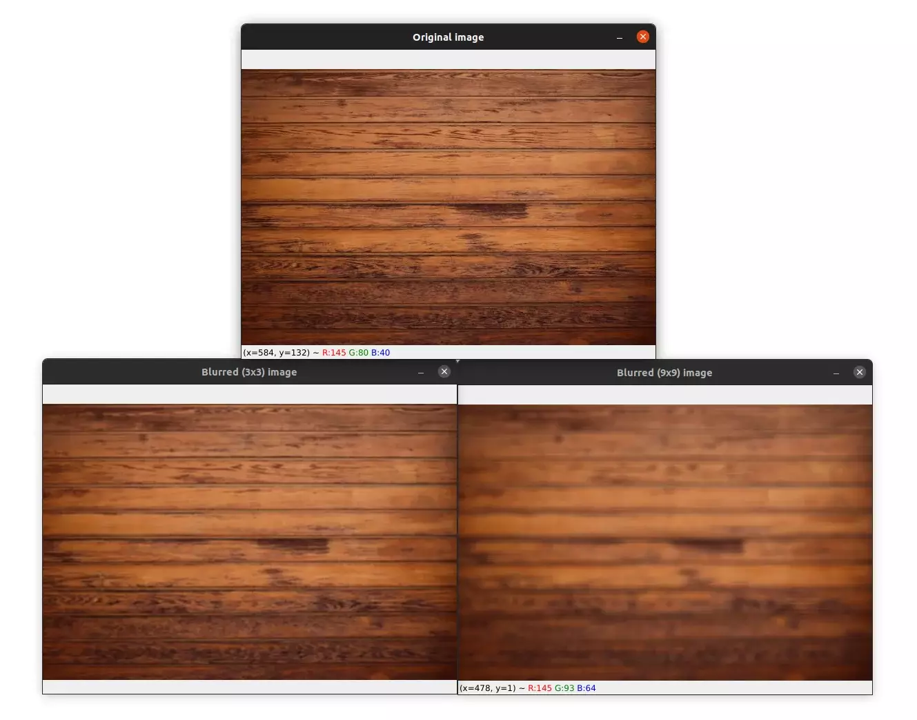
Notice how the filtered images with a kernel size of 3x3 and 9x9 have been blurred compared to the original image. You can see that with a kernel size of 9x9 the image is more blurred than with a 3x3 kernel.
Gaussian Blurring
Let's now see Gaussian blurring. As the name suggests, this technique uses a Gaussian distribution to construct the kernel.
As opposed to the first example, where we used a simple average, Gaussian blurring applies a weighted average, where pixels that are closer to the center of the kernel have more weight than pixels that are further away.
Let's see now Gaussian blurring with an example:
image = cv2.imread("wood.jpg")
cv2.imshow("Original image", image)

gaussian_blur_3x3 = cv2.GaussianBlur(image, (3, 3), 0)
cv2.imshow("Gaussian blur (3x3)", gaussian_blur_3x3)

gaussian_blur_9x9 = cv2.GaussianBlur(image, (9, 9), 0)
cv2.imshow("Gaussian blur (9x9)", gaussian_blur_9x9)

cv2.waitKey(0)
The cv2.GaussianBlur function applies a Gaussian blur to our image. The first argument to this function is the input image we want to blur. The second argument is a tuple to specify the kernel size.
The last parameter is the standard deviation of the Gaussian distribution. By using a value of 0, the standard deviation will be computed from the kernel size.
The result of Gaussian blurring is shown below:
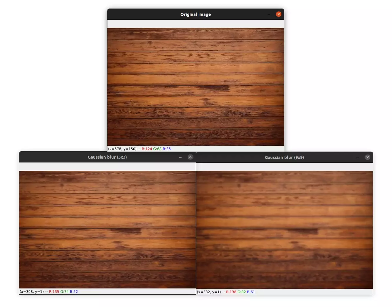
As you can see, Gaussian blurring preserves the edges of the image better than with average blurring.
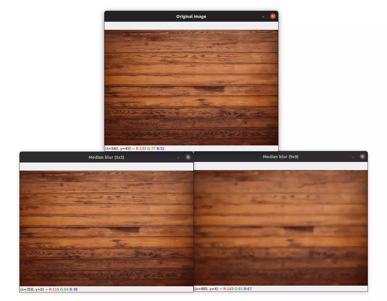
Median Blurring
Median blurring is often used to remove "salt and pepper" in an image. Each pixel in the input image is replaced with the median of all other pixels surrounding it (pixels in the kernel area).
Let's see an example of median blurring:
image = cv2.imread("wood.jpg")
cv2.imshow("Original image", image)

median_blur_3x3 = cv2.medianBlur(image, 3)
cv2.imshow("Median blur (3x3)", median_blur_3x3)

median_blur_9x9 = cv2.medianBlur(image, 9)
cv2.imshow("Median blur (9x9)", median_blur_9x9)

cv2.waitKey(0)
To apply median blurring we use the cv2.medianBlur function. This function takes the image we want to blur as a first parameter and the kernel size as a second parameter. Please note that the kernel size must be square.
You can see the output of the median blur in the image below:
Bilateral Blurring
As we saw in the previous examples, the purpose of blurring is to reduce the noise and unnecessary detail in an image but this can result in the loss of the edges.
To preserve edges, bilateral blurring replaces each pixel intensity with the weighted average of the neighborhood pixels, where pixels that are closer to the center of the kernel are given more weights. But it also considers the variation in the intensities of neighboring pixels ensuring that the computation of the blur only includes pixels of similar intensity.
Let's see an example of bilateral blurring:
image = cv2.imread("wood.jpg")
cv2.imshow("Original image", image)

bilateral_blur1 = cv2.bilateralFilter(image, 11, 21, 11)
cv2.imshow("Bilateral blur (11, 21, 11)", bilateral_blur1)

bilateral_blur2 = cv2.bilateralFilter(image, 15, 51, 29)
cv2.imshow("Bilateral blur (15, 51, 29)", bilateral_blur2)

cv2.waitKey(0)
Bilateral blurring is applied using the cv2.bilateralFilter function. As always, the first argument to this function is the image we want to blur.
The second argument is the diameter of the pixel neighborhood used for the computation of the blur.
The third parameter, sigmaColor, defines the standard deviation of the color intensity, which means that the larger the value for this parameter the more difference in pixel intensity will be tolerated.
The last argument, sigmaSpace, specifies the space standard deviation (just like with the GaussianBlur function). A larger value for this parameter means that pixels farther from the center of the kernel size will have an influence in the computation of the blur.
The output of bilateral blurring is shown below:
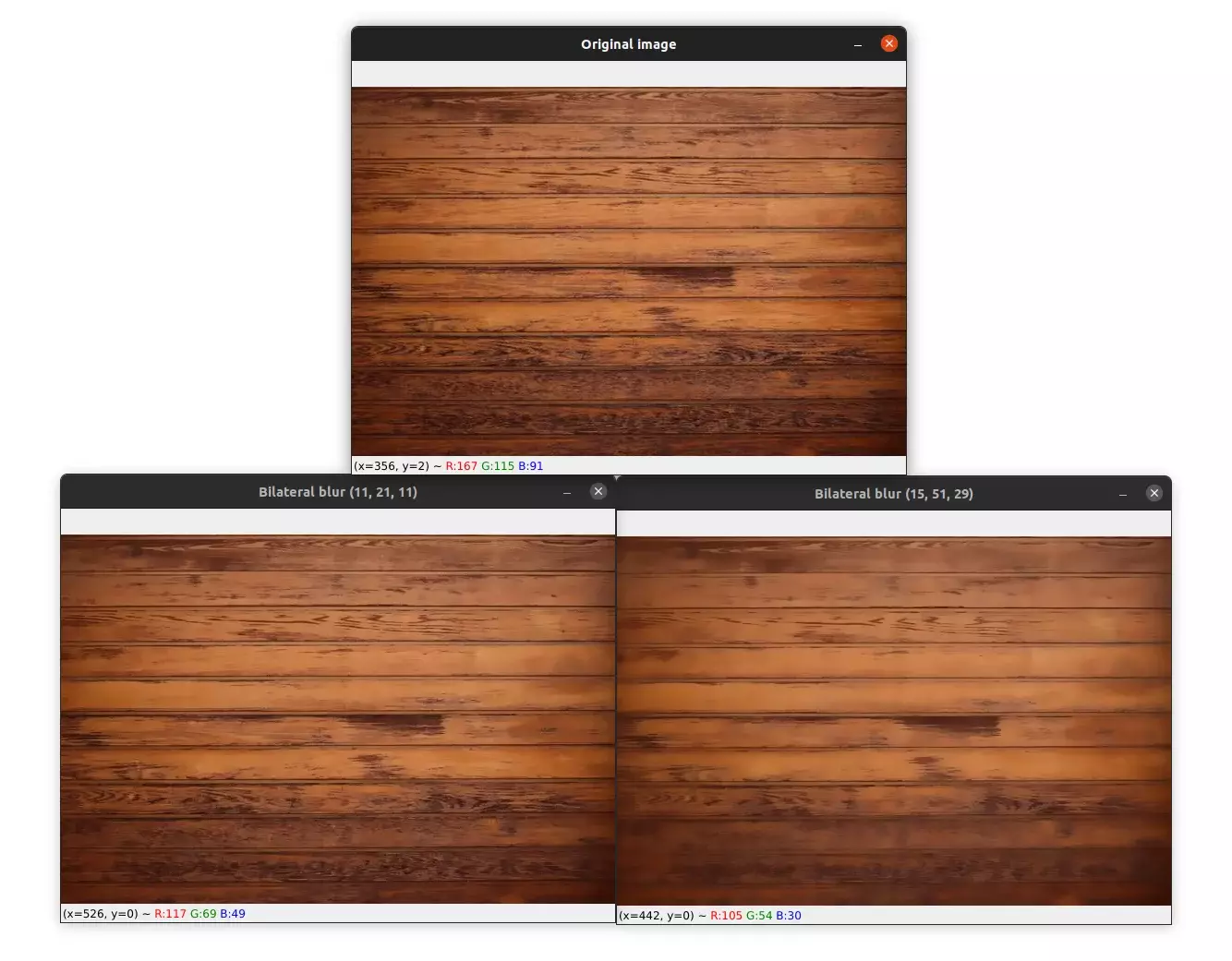
You can see that regions of similar pixels intensity have been smoothed (blurred), on the other hand, the cracks in the wood (the edges) have been preserved.
The downside of this technique is that it is very computationally expensive compared to the other techniques.
Summary
In this tutorial, you learned four different techniques of blurring. Take the time to explore each one because we are going to use blurring in the tutorial part where we introduce thresholding.
If you want to learn more about computer vision and image processing then check out my course Computer Vision and Image Processing with OpenCV and Python.
Previous Article
Face Detection and Blurring with OpenCV and Python
Next Article
YOLOv4 Custom Object Detection with OpenCV and Python
@Ngoc to check the image results you need to display the image and compare it with the original one.

It's not really un percentage of blur that we apply. it is rather a mathematical operation (a convolution) which is applied to the original image.
If we want a very blurry image, we apply a filter with a very large kernel size.

Image blurring is generally applied as a preprocessing or image augmentation step before feeding the image to a machine learning model.

Please read this article for more information: https://blog.roboflow.com/using-blur-in-computer-vision-preprocessing/
Nov. 30, 2022, 10:14 p.m.
Nov. 30, 2022, 2:14 p.m.